Aloof as stardust rains
Are memory dim prints
Eliding tensed face
By shadows within of
All conquering space that
Inly trusts each friend
Of madness—whose embrace
Accept with no delays
To take one final look
Before you turn Rose ways.
A rather rare meter in English, but much easier once you let enjambments in.
Précis
3-LISP is a dialect of LISP designed and implemented by Brian C. Smith as part of his PhD. thesis Procedural Reflection in Programming Languages (what this thesis refers to as "reflection" is nowadays more usually called "reification"). A 3-LISP program is conceptually executed by an interpreter written in 3-LISP that is itself executed by an interpreter written in 3-LISP and so on ad infinitum. This forms a (countably) infinite tower of meta-circular (v.i.) interpreters. reflective lambda is a function that is executed one tower level above its caller. Reflective lambdas provide a very general language extension mechanism.
The code is here.
Meta-circular interpreters
An interpreter is a program that executes programs written in some programming language.
A meta-circular interpreter is an interpreter for a programming language written in that language. Meta-circular interpreters can be used to clarify or define the semantics of the language by reducing the full language to a sub-language in which the interpreter is expressed. Historically, such definitional interpreters become popular within the functional programming community, see the classical Definitional interpreters for higher-order programming languages. Certain important techniques were classified and studied in the framework of meta-circular interpretation, for example, continuation passing style can be understood as a mechanism that makes meta-circular interpretation independent of the evaluation strategy: it allows an eager meta-language to interpret a lazy object language and vice versa. As a by-product, a continuation passing style interpreter is essentially a state machine and so can be implemented in hardware, see The Scheme-79 chip. Similarly, de-functionalisation of languages with higher-order functions obtains for them first-order interpreters. But meta-circular interpreters occur in imperative contexts too, for example, the usual proof of the Böhm–Jacopini theorem (interestingly, it was Corrado Böhm who first introduced meta-circular interpreters in his 1954 PhD. thesis) constructs for an Algol-like language a meta-circular interpreter expressed in some goto-less subset of the language and then specialises this interpreter for a particular program in the source language.
Given a language with a meta-circular interpreter, suppose that the language is extended with a mechanism to trap to the meta-level. For example, in a LISP-like language, that trap can be a new special form (reflect FORM) that directly executes (rather than interprets) FORM within the interpreter. Smith is mostly interested in reflective (i.e., reification) powers obtained this way, and it is clear that the meta-level trap provides a very general language extension method: one can add new primitives, data types, flow and sequencing control operators, etc. But if you try to add reflect to an existing LISP meta-circular interpreter (for example, see p. 13 of LISP 1.5 Programmers Manual) you'd hit a problem: FORM cannot be executed at the meta-level, because at this level it is not a form, but an S-expression.
Meta-interpreting machine code
To understand the nature of the problem, consider a very simple case: the object language is the machine language (or equivalently the assembly language) of some processor. Suppose that the interpreter for the machine code is written in (or, more realistically, compiled to) the same machine language. The interpreter maintains the state of the simulated processor that is, among other things registers and memory. Say, the object (interpreted) code can access a register, R0, then the interpreter has to keep the contents of this register somewhere, but typically not in its (interpreter's) R0. Similarly, a memory word visible to the interpreted code at an address ADDR is stored by the interpreter at some, generally different, address ADDR' (although, by applying the contractive mapping theorem and a lot of hand-waving one might argue that there will be at least one word stored at the same address at the object- and meta-levels). Suppose that the interpreted machine language has the usual sub-routine call-return instructions call ADDR and return and is extended with a new instruction reflect ADDR that forces the interpreter to call the sub-routine ADDR. At the very least the interpreter needs to convert ADDR to the matching ADDR'. This might not be enough because, for example, the object-level sub-routine ADDR might not be contiguous at the meta-level, i.e., it is not guaranteed that if ADDR maps to ADDR' then (ADDR + 1) maps (ADDR' + 1). This example demonstrates that a reflective interpreter needs a systematic and efficient way of converting or translating between object- and meta-level representations. If such a method is somehow provided, reflect is a very powerful mechanism: by modifying interpreter state and code it can add new instructions, addressing modes, condition bits, branch predictors, etc.
N-LISP for a suitable value of N
In his thesis Prof. Smith analyses what would it take to construct a dialect of LISP for which a faithful reflective meta-circular interpreter is possible. He starts by defining a formal model of computation with an (extremely) rigorous distinction between meta- and object- levels (and, hence, between use and mention). It is then determined that this model can not be satisfactorily applied to the traditional LISP (which is called 1-LISP in the thesis and is mostly based on Maclisp). The reason is that LISP's notion of evaluation conflates two operations: normalisation that operates within the level and reference that moves one level down. A dialect of LISP that consistently separates normalisation and reference is called 2-LISP (the then new Scheme is called 1.75-LISP). Definition of 2-LISP occupies the bulk of the thesis, which the curious reader should consult for (exciting, believe me) details.
Once 2-LISP is constructed, adding the reflective capability to it is relatively straightforward. Meta-level trap takes the form of a special lambda expression:
(lambda reflect [ARGS ENV CONT] BODY)When this lambda function is applied (at the object level), the body is directly executed (not interpreted) at the meta-level with ARGS bound to the meta-level representation of the actual parameters, ENV bound to the environment (basically, the list of identifiers and the values they are bound to) and CONT bound to the continuation. Environment and continuation together represent the 3-LISP interpreter state (much like registers and memory represent the machine language interpreter state), this representation goes all the way back to SECD machine, see The Mechanical Evaluation of Expressions.
Here is the fragment of 3-LISP meta-circular interpreter code that handles lambda reflect (together with "ordinary" lambda-s, denoted by lambda simple):
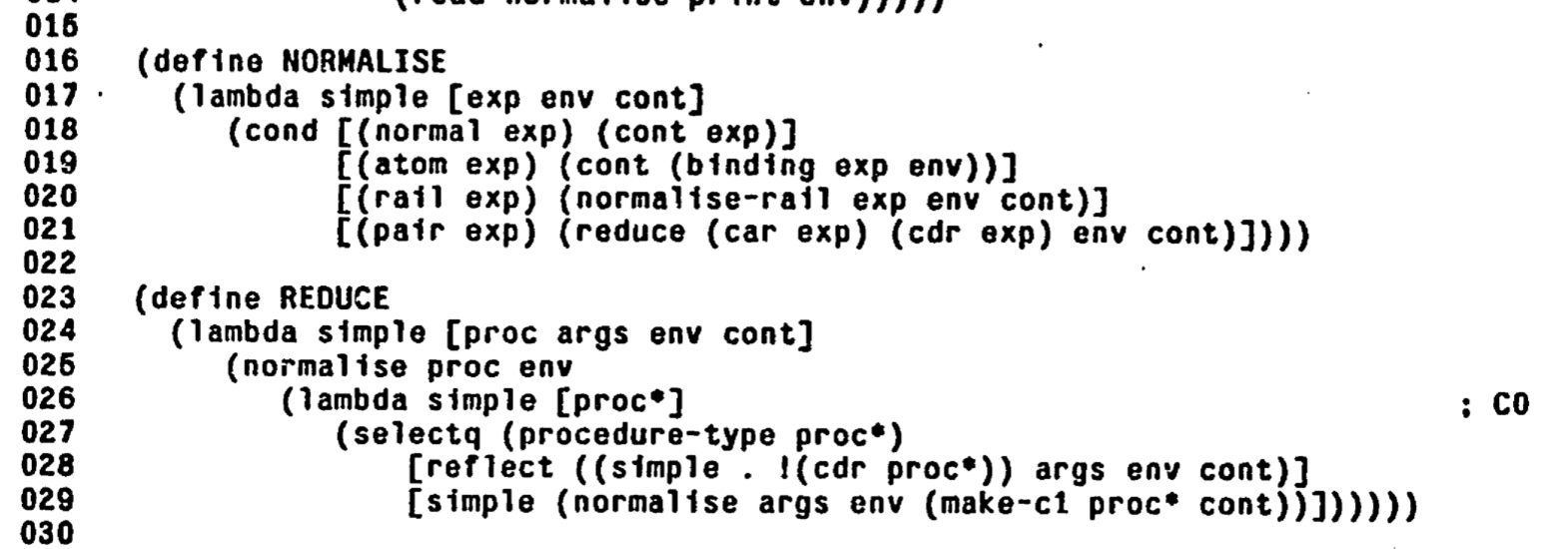
Implementation
It is of course not possible to run an infinite tower of interpreters directly.
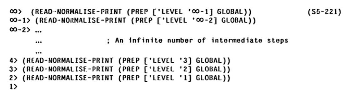
3-LISP implementation creates a meta-level on demand, when a reflective lambda is invoked. At that moment the state of the meta-level interpreter is synthesised (e.g., see make-c1 in the listing above). The implementation takes pain to detect when it can drop down to a lower level, which is not entirely simple because a reflective lambda can, instead of returning (that is, invoking the supplied continuation), run a potentially modified version of the read-eval-loop (called READ-NORMALISE-PRINT in 3-LISP) which does not return. There is a lot of non-trivial machinery operating behind the scenes and though the implementation modestly proclaims itself extremely inefficient it is, in fact, remarkably fast.
Porting
I was unable to find a digital copy of the 3-LISP sources and so manually retyped the sources from the appendix of the thesis. The transcription in 3-lisp.lisp (2003 lines, 200K characters) preserves the original pagination and character set, see the comments at the top of the file. Transcription was mostly straightforward except for a few places where the PDF is illegible (for example, see here) all of which fortunately are within comment blocks.
The sources are in CADR machine dialect of LISP, which, save for some minimal and no longer relevant details, is equivalent to Maclisp.
3-LISP implementation does not have its own parser or interpreter. Instead, it uses flexibility built in a LISP reader (see, readtables) to parse, interpret and even compile 3-LISP with a very small amount of additional code. Amazingly, this more than 40 years old code, which uses arcane features like readtable customisation, runs on a modern Common Lisp platform after a very small set of changes: some functions got renamed (CASEQ to CASE, *CATCH to CATCH, etc.), some functions are missing (MEMQ, FIXP), some signatures changed (TYPEP, BREAK, IF). See 3-lisp.cl for details.
Unfortunately, the port does not run on all modern Common Lisp implementations, because it relies on the proper support for backquotes across recursive reader invocations:
;;     Maclisp maintains backquote context across recursive parser
;;     invocations. For example in the expression (which happens within defun
;;     3-EXPAND-PAIR)
;;
;;         `\(PCONS ~,a ~,d)
;;
;;     the backquote is consumed by the top-level activation of READ. Backslash
;;     forces the switch to 3-lisp readtable and call to 3-READ to handle the
;;     rest of the expression. Within this 3-READ activation, the tilde forces
;;     switch back to L=READTABLE and a call to READ to handle ",a". In Maclisp,
;;     this second READ activation re-uses the backquote context established by
;;     the top-level READ activation. Of all Common Lisp implementations that I
;;     tried, only sbcl correctly handles this situation. Lisp Works and clisp
;;     complain about "comma outside of backquote". In clisp,
;;     clisp-2.49/src/io.d:read_top() explicitly binds BACKQUOTE-LEVEL to nil.
Among Common Lisp implementations I tried, only sbcl supports it properly. After reading Common Lisp Hyperspec, I believe that it is Maclisp and sbcl that implement the specification correctly and other implementations are faulty.
Conclusion
Procedural Reflection in Programming Languages is, in spite of its age, a very interesting read. Not only does it contain an implementation of a refreshingly new and bold idea (it is not even immediately obvious that infinite reflective towers can at all be implemented, not to say with any reasonable degree of efficiency), it is based on an interplay between mathematics and programming: the model of computation is proposed and afterward implemented in 3-LISP. Because the model is implemented in an actual running program, it has to be specified with extreme precision (which would make Tarski and Łukasiewicz tremble), and any execution of the 3-LISP interpreter validates the model.
„adaptive replacement better than Working Set?“ has (an implicit) idea: VM page replacement should keep a spectrum of accesses to a given page. Too high and too low frequences should be filtered out, because they:
represent correlated references, and
irrelevant,
respectively.
Groups usually come with homomorphisms, defined as mappings preserving multiplication:
$$f(a\cdot b) = f(a)\cdot f(b)$$From this definition, notions of subgroup (monomorphism), quotient group (epimorphism, normal subgroup) and the famous isomorphism theorem follow naturally. The category of groups with homomorphisms as arrows has products and sums, equalizers and coequalizers all well-known and with nice properties.
Consider, instead, affine morphism, that can be defined by the following equivalent conditions:
1. \(f(a \cdot b^{-1} \cdot c) = f(a) \cdot f^{-1}(b) \cdot f(c)\)
2. \(f(a \cdot b) = f(a) \cdot f^{-1}(e) \cdot f(b)\)
3. \(\exists t. f(a \cdot b) = f(a) \cdot t \cdot f(b)\)
The motivation for this definition is slightly roundabout.
The difference between homomorphism and affine morphism is similar to the difference between a vector subspace and an affine subspace of a vector space. A vector subspace always goes through the origin (for a homomorphism \(f\), \(f(e) = e\)), whereas an affine subspace is translated from the origin (\(f(e) \neq e\) is possible for an affine morphism).
Take points \(f(a)\) and \(f(b)\) in the image of an affine morphism, translate them back to the corresponding "vector subspace" to obtain \(f(a) \cdot f^{-1}(e)\) and \(f(b) \cdot f^{-1}(e)\). If translated points are multiplied and the result is translated back to the affine image, the resulting point should be the same as \(f(a \cdot b)\):
$$f(a \cdot b) = (f(a) \cdot f^{-1}(e)) \cdot (f(b) \cdot f^{-1}(e)) \cdot f(e) = f(a) \cdot f^{-1}(e) \cdot f(b)$$which gives the definition (2).
(1) => (2) immediately follows by substituting \(e\) for \(b\).
(2) => (3) by substituting \(f^{-1}(e)\) for \(t\).
(3) => (2) by substituting \(e\) for \(a\) and \(b\).
(2) => (1)
$$\begin{array}{r@{\;}c@{\;}l@{\quad}l@{\quad}} f(a \cdot b^{-1} \cdot c) &\;=\;& & \\ &\;=\;& f(a) \cdot f^{-1}(e) \cdot f(b^{-1} \cdot c) & \text{\{(2) for \(a \cdot (b^{-1} \cdot c)\)\}} \\ &\;=\;& f(a) \cdot f^{-1}(e) \cdot f(b^{-1}) \cdot f^{-1}(e) \cdot f(c) & \text{\{(2) for \(b^{-1} \cdot c\)\}} \\ &\;=\;& f(a) \cdot f^{-1}(e) \cdot f(b^{-1}) \cdot f^{-1}(e) \cdot f(b) \cdot f^{-1}(b) \cdot f(c) & \text{\{\(e = f(b) \cdot f^{-1}(b)\), working toward } \\ & & & \text{creating a sub-expression that can be collapsed by (2)\}} \\ &\;=\;& f(a) \cdot f^{-1}(e) \cdot f(b^{-1} \cdot b) \cdot f^{-1}(b) \cdot f(c) & \text{\{collapsing \(f(b^{-1}) \cdot f^{-1}(e) \cdot f(b)\) by (2)\}} \\ &\;=\;& f(a) \cdot f^{-1}(e) \cdot f(e) \cdot f^{-1}(b) \cdot f(c) & \text{\{\(b^{-1} \cdot b = e\)\}} \\ &\;=\;& f(a) \cdot f^{-1}(b) \cdot f(c) & \text{\{\(f^{-1}(e) \cdot f(e) = e\)\}} \end{array}$$It is easy to check that each homomorphism is an affine morphism (specifically, homomorphisms are exactly affine morphisms with \(f(e) = e\)).
Composition of affine morphisms is affine and hence groups with affine morphisms form a category \(\mathbb{Aff}\).
A subset of a group \(G\) is called an affine subgroup of \(G\) if one of the following equivalent conditions holds:
1. \(\exists h \in G:\forall p, q \in H \rightarrow (p \cdot h^{-1} \cdot q \in H \wedge h \cdot p^{-1} \cdot h \in H)\)
2. \(\forall p, q, h \in H \rightarrow (p \cdot h^{-1} \cdot q \in H \wedge h \cdot p^{-1} \cdot h \in H)\)
The equivalence (with a proof left as an exercise) means that if any \(h\) "translating" affine subgroup to a subgroup exists, then any member of the affine subgroup can be used for translation. In fact, any \(h\) that satisfies (1) belongs to \(H\) (prove). This matches the situation with affine and vector subspaces: any vector from an affine subspace translates this subspace to the subspace passing through the origin.
Finally for to-day, consider an affine morphism \(f:G_0\rightarrow G_1\). For \(t\in G_0\) define kernel:
$$ker_t f = \{g\in G_0 | f(g) = f(t)\}$$It's easy to check that a kernel is affine subgroup (take \(t\) as \(h\)). Note that in \(\mathbb{Aff}\) a whole family of subobjects corresponds to a morphism, whereas there is the kernel in \(\mathbb{Grp}\).
To be continued: affine quotients, products, sums, free affine groups.
Already in 1956 it was clear that one had to work with symbolic expressions to reach the goal of artifical intelligence. As the researchers already understood numerical computation would not have much importance.
-- Early LISP History (1956 - 1959)
Here is a little problem. Given an array \(A\) of \(N\) integers, find a sub-array (determined by a pair of indices within \(A\)) such that sum of elements in that sub-array is maximal among all sub-arrays of \(A\).
Sounds pretty easy? It is, but just to set a little standard for solutions: there is a way (shown to me by a 15-year-old boy) to do this in one pass over \(A\) and without using any additional storage except for few integer variables.
So much for dynamic programming...
update
That exercise is interesting, because while superfluously similar to the well-known tasks like finding longest common substring, etc. it can be solved in one pass.
Indeed Matti presented exactly the same solution that I had in mind. And it is possible (and instructive) to get a rigorous proof that this algorithm solves the problem.
Definition 0. Let \(A = (i, j)\) be a sub-array \((i <= j)\), then \(S(A) = S(i, j)\) denotes a sum of elements in \(A\). \(S(A)\) will be called sum of \(A\).
Definition 1. Let \(A = (i, j)\) be a sub-array \((i <= j)\), then for any
$$0 <= p < i < q < j < r < N$$sub-array \((p, i - 1)\) is called left outfix of \(A\), \((i, q)\) --- left infix of \(A\), \((q + 1, j)\) --- right infix of \(A\), and \((j + 1, r)\) --- right outfix of \(A\).
Definition 2. A sub-array is called optimal if all its infixes have positive sums, and all its outfixes have negative sums.
It's easy to prove the following:
Statement 0. A sub-array with the maximal sum is optimal.
Indeed, any non-optimal sub-array by definition has either negative infix, or positive outfix, and, hence, can be shrunken or expanded to another sub-array that has larger sum.
As an obvious corollary we get:
Statement 1. To find a sub-array with the maximal sum it's enough to find a sub-array with the maximal sum among all optimal sub-arrays.
The key fact that explains why our problem can be solved in one pass is captured in the following:
Statement 2. Optimal sub-arrays are not overlapping.
Also easily proved by observing that when two sub-arrays \(A\) and \(B\) overlap there always is an sub-array \(C\) that is an infix of \(A\) and an outfix of \(B\).
And, now the only thing left to do is to prove that Matti's algorithm calculates sums of (at least) all optimal sub-arrays. Which is easy to do:
first prove that possibly except for the initial value, new_start always points to the index at which at least one (and, therefore, exactly one) optimal array starts. This is easily proved by induction.
then prove that once particular value of new_start has been reached, new_start is not modified until i reaches upper index of optimal array starting at new_start. This follows directly from the definition of optimal sub-array, because all its left infixes have positive sums.
this means that for any optimal sub-array \((p, q)\) there is an iteration of the loop at which
$$new\_start == p \quad\text{and}\quad i == q$$As algorithm finds maximal sum among all \((new\_start, i)\) sub-arrays, it finds maximal sum among all optimal arrays, and, by Statement 1, maximal sum among all sub-arrays.
\( \def\List{\operatorname{List}} \) \( \def\integer{\operatorname{integer}} \) \( \def\nat{\operatorname{nat}} \) \( \def\Bool{\operatorname{Bool}} \) \( \def\Punct{\operatorname{Punct}} \) \( \def\BT{\operatorname{BT}} \) \( \def\B{\operatorname{B}} \) \( \def\T{\operatorname{T}} \) \( \def\R{\operatorname{R}} \) \( \def\Set{\operatorname{Set}} \) \( \def\Bag{\operatorname{Bag}} \) \( \def\Ring{\operatorname{Ring}} \) \( \def\plug{\operatorname{plug}} \) \( \def\Zipper{\operatorname{Zipper}} \) \( \def\cosh{\operatorname{cosh}} \) \( \def\sinh{\operatorname{sinh}} \) \( \def\ch{\operatorname{ch}} \) \( \def\sh{\operatorname{sh}} \) \( \def\d{\partial} \)
There is that curious idea that you can think of a type in a programming language as a kind of algebraic object. Take (homogeneous) lists for example. A list of integers is either an empty list (i.e., nil) or a pair of an integer (the head of the list) and another list (the tail of the list). You can symbolically write this as
Here \(1\) is the unit type with one element, it does not matter what this element is exactly. \(A + B\) is a disjoint sum of \(A\) and \(B\). It is a tagged union type, whose values are values of \(A\) or \(B\) marked as such. \(A \cdot B\) is the product type. Its values are pairs of values of \(A\) and \(B\).
The underlying mathematical machinery includes "polynomial functors", "monads", "Lambek's theorem", etc. You can stop digging when you reach "Knaster-Tarski theorem" and "Beck's tripleability condition".
In general, we have
$$\List(x) = 1 + x \cdot \List(x)$$In Haskell this is written as
data List x = Nil | Cons x (List x)Similarly, a binary tree with values of type \(x\) at the nodes can be written as
$$\BT(x) = 1 + x\cdot \BT(x) \cdot \BT(x)$$That is, a binary tree is either empty or a triple of the root, the left sub-tree and the right sub-tree. If we are only interested in the "shapes" of the binary trees we need
$$\B = \BT(1) = 1 + \B^2$$Nothing too controversial so far. Now, apply some trivial algebra:
$$\begin{array}{r@{\;}c@{\;}l@{\quad}} \List(x) &\;=\;& 1 + x \cdot \List(x) \\ \List(x) - x \cdot \List(x) &\;=\;& 1 \\ \List(x) \cdot (1 - x) &\;=\;& 1 \\ \List(x) &\;=\;& \frac{1}{1 - x} \\ \List(x) &\;=\;& 1 + x + x^2 + x^3 + \cdots \end{array}$$Going from \(\List(x) - x \cdot \List(x)\) to \(\List(x) \cdot (1 - x)\) in the middle step arguably makes some sense: product of sets and types distributes over sum, much like it does for integers. But the rest is difficult to justify or even interpret. What is the difference of types or their infinite series?
The last equation, however, is perfectly valid: an element of \(\List(x)\) is either nil, or a singleton element of \(x\), or a pair of elements of \(x\) or a triple, etc. This is somewhat similar to the cavalier methods of eighteenth-century mathematicians like Euler and the Bernoulli brothers, who would boldly go where no series converged before and through a sequence of meaningless intermediate steps arrive to a correct result.
One can apply all kinds of usual algebraic transformations to \(\List(x) = (1 - x)^{-1}\). For example,
$$\begin{array}{r@{\;}c@{\;}l@{\quad}l@{\quad}} \List(a + b) &\;=\;& \frac{1}{1 - a - b} \\ &\;=\;& \frac{1}{1 - a}\cdot\frac{1}{1 - \frac{b}{1 - a}} \\ &\;=\;& \List(a)\cdot\List(\frac{b}{1 - a}) \\ &\;=\;& \List(a)\cdot\List(b\cdot\List(a)) \end{array}$$This corresponds to the regular expressions identity \((a|b)^* = a^*(ba^*)^*\).
Apply the same trick to binary trees:
$$\begin{array}{r@{\;}c@{\;}l@{\quad}l@{\quad}} \BT &\;=\;& 1 + \BT^2 \cdot x & \\ \BT^2 \cdot x - \BT + 1 &\;=\;& 0 & \text{(Solve the quadratic equation.)} \\ \BT &\;=\;& \frac{1\pm\sqrt{1-4\cdot x}}{2\cdot x} & \text{(Use binomial theorem)} \\ \sqrt{1-4\cdot x} &\;=\;& \sum_{k=0}^\infty \binom{\tfrac12}{k}(-4\cdot x)^k & \\ \BT(x) &\;=\;& 1 + x + 2\cdot x^2 + 5\cdot x^3 + 14\cdot x^4 + 42\cdot x^5 + \cdots & \\ &\;=\;& \sum_{n=0}^\infty C_n\cdot x^n, & \end{array}$$Where \(C_n=\frac{1}{n+1}\binom{2\cdot n}{n}\)—the \(n\)-th Catalan number, that is the number of binary trees with \(n\) nodes. To understand the last series we need to decide what \(n\cdot x\) is, where \(n\) is a non-negative integer and \(x\) is a type. Two natural interpretations are
$$n \cdot x = x + x + \cdots = \sum_0^{n - 1} x$$and
$$n \cdot x = \{0, \ldots, n - 1\} \cdot x$$which both mean the same: an element of \(n\cdot x\) is an element of \(x\) marked with one of \(n\) "branches", and this is the same as a pair \((i, t)\) where \(0 <= i < n\) and \(t\) is an element of \(x\).
The final series then shows that a binary tree is either an empty tree (\(1\)) or an \(n\)-tuple of \(x\)-es associated with one of \(C_n\) shapes of binary trees with \(n\) nodes. It worked again!
Now, watch carefully. Take simple unmarked binary trees: \(\B = \BT(1) = 1 + \B^2\). In this case, we can "calculate" the solution exactly:
$$\B^2 - \B + 1 = 0$$hence
$$\B = \frac{1 \pm \sqrt{1 - 4}}{2} = \frac{1}{2} \pm i\cdot\frac{3}{2} = e^{\pm i\cdot\frac{\pi}{3}}$$Both solutions are sixth-degree roots of \(1\): \(\B^6 = 1\). OK, this is still completely meaningless, right? Yes, but it also means that \(\B^7 = \B\), which --if correct-- would imply that there is a bijection between the set of all binary trees and the set of all 7-tuples of binary trees. Haha, clearly impossible... Actually, it's a more or less well-known fact.
A note is in order. All "sets" and "types" that we talked about so far are at most countably infinite so, of course, there exists a bijection between \(\B\) and \(\B^7\) simply because both of these sets are countable. What is interesting, and what the paper linked to above explicitly establishes, is that there is as they call it "a very explicit" bijection between these sets, that is a "structural" bijection that does not look arbitrarily deep into its argument trees. For example, in a functional programming language, such a bijection can be coded through pattern matching without recursion.
Here is another neat example. A rose tree is a kind of tree datatype where a node has an arbitrary list of children:
$$\R(x) = x\cdot\List(\R(x))$$Substituting \(\List(x) = (1 - x)^{-1}\) we get
$$\R(x) = \frac{x}{1 - R(x)}$$or
$$\R^2(x) - \R(x) + x = 0$$Hence \(\R = \R(1)\) is defined by the same equation as \(\B = \BT(1)\): \(\R^2 - \R + 1 = 0\). So, there must be a bijection between \(\R\) and \(\B\), and of course there is: one of the first things LISP hackers realised in the late 1950s is that an arbitrary tree can be encoded with cons cells.
Mathematically, this means that instead of "initial algebras" we treat types as "final co-algebras".
All this is, by the way, is equally applicable to infinite datatypes (that is, streams, branching transition systems, etc.)
That was pure algebra, there is nothing "analytical" here. Analysis historically started with the notion of derivative. And sure, you can define and calculate derivatives of data type constructors like \(\List\) and \(\BT\). These derivatives are generalisations of zipper-like structures: they represent "holes" in the data-type, that can be filled by an instance of the type-parameter.
For example, suppose you have a list \((x_0, \ldots, x_k, \ldots, x_{n - 1})\) of type \(\List(x)\) then a hole is obtained by cutting out the element \(x_k\) that is \((x_0, \ldots, x_{k-1}, \blacksquare, x_{k+1}, \ldots, x_{n - 1})\) and is fully determined by the part of the list to the left of the hole \((x_0, \ldots, x_{k - 1})\) and the part to the right \((x_{k+1}, \ldots, x_{n - 1})\). Both of these can be arbitrary lists (including empty), so a hole is determined by a pair of lists and we would expect \(\d \List(x) = \List^2(x)\). But Euler would have told us this immediately, because \(\List(x) = (1 - x)^{-1}\) hence
$$\d \List(x) = \d (1 - x)^{-1} = (1 - x)^{-2} = \List^2(x)$$In general the derivative of a type constructor (of a "function" analytically speaking) \(T(x)\) comes with a "very explicit" surjective function
$$\plug : \d T(x) \cdot x \to T(x)$$injective on each of its arguments, and has the usual properties of a derivative, among others:
$$\begin{array}{r@{\;}c@{\;}l@{\quad}} \d (A + B) &\;=\;& \d A + \d B \\ \d (A \cdot B) &\;=\;& \d A \cdot B + A \cdot \d B \\ \d_x A(B(x)) &\;=\;& \d_B A(B) \cdot \d_x B(x) \\ \d x &\;=\;& 1 \\ \d x^n &\;=\;& n\cdot x^{n-1} \\ \d n &\;=\;& 0 \end{array}$$For binary trees we get
$$\begin{array}{r@{\;}c@{\;}l@{\quad}} \d \BT(x) &\;=\;& \d (1 + x\cdot \BT^2(x)) \\ &\;=\;& 0 + \BT^2(x) + 2\cdot x\cdot \BT(x) \cdot \d \BT(x) \\ &\;=\;& \BT^2(x) / (1 - 2\cdot x\cdot \BT(x)) \\ &\;=\;& \BT^2(x) \cdot \List(2\cdot x\cdot \BT(x)) \\ &\;=\;& \BT^2(x) \cdot \Zipper_2(x) \end{array}$$Here \(\Zipper_2(x) = \List(2\cdot x\cdot \BT(x))\) is the classical Huet's zipper for binary trees. We have an additional \(\BT^2(x)\) multiplier, because Huet's zipper plugs an entire sub-tree, that is, it's a \(\BT(x)\)-sized hole, whereas our derivative is an \(x\)-sized hole.
For \(n\)-ary trees \(\T = 1 + x\cdot \T^n(x)\) we similarly have
$$\begin{array}{r@{\;}c@{\;}l@{\quad}} \d \T(x) &\;=\;& \d (1 + x\cdot \T^n(x)) \\ &\;=\;& 0 + \T^n(x) + n\cdot x\cdot \T^{n-1}(x) \cdot \d \T(x) \\ &\;=\;& \T^n(x) / (1 - n\cdot x\cdot \T^{n -1}(x)) \\ &\;=\;& \T^n(x) \cdot \List(n\cdot x\cdot \T^{n - 1}(x)) \\ &\;=\;& \T^n(x) \cdot \Zipper_n(x) \end{array}$$At this point we have basic type constructors for arrays (\(x^n\)), lists and variously shaped trees, which we can combine and compute their derivatives. We can also try constructors with multiple type parameters (e.g., trees with different types at the leaves and internal nodes) and verify that the usual partial-differentiation rules apply. But your inner Euler must be jumping up and down: much more is possible!
Indeed it is. Recall the "graded" representation of \(\List(x)\):
$$\List(x) = 1 + x + x^2 + x^3 + \cdots$$This formula says that there is one (i.e, \(|x|^0\)) list of length \(0\), one list (of length \(1\)) for each element of \(x\), one list for each ordered pair of elements of \(x\), for each ordered triple, etc. What if we forget the order of \(n\)-tuples? Then, by identifying each of the possible \(n!\) permutations, we would get, instead of lists with \(n\) elements, multisets (bags) with \(n\) elements.
$$\Bag(x) = \frac{1}{0!} + \frac{x}{1!} + \frac{x^2}{2!} + \cdots + \frac{x^k}{k!} + \cdots = e^x$$[0]
Formally we move from polynomial functors to "analytic functors" introduced by A. Joyal.
This counting argument, taken literally, does not hold water. For one thing, it implies that every term in \(e^x\) series is an integer (hint: there are no \(n!\) \(n\)-tuples belonging to the same class as \((t, t, \ldots, t)\)). But it drives the intuition in the right direction and \(\Bag(x)\) does have the same properties as the exponent. Before we demonstrate this, let's look at another example.
A list of \(n\) elements is one of \(|x|^n\) \(n\)-tuples of elements of \(x\). A bag with \(n\) elements is one of such tuples, considered up to a permutation. A set with \(n\) elements is an \(n\)-tuple of different elements considered up to a permutation. Hence, where for lists and bags we have \(x^n\), sets have \(x\cdot(x - 1)\cdot\cdots\cdot(x - n + 1)\) by the standard combinatorial argument: there are \(x\) options for the first element, \(x - 1\) options for the second element and so on.
That is,
$$\begin{array}{r@{\;}c@{\;}l@{\quad}} \Set(x) &\;=\;& 1 + \frac{x}{1!} + \frac{x\cdot(x - 1)}{2!} + \frac{x\cdot(x - 1)\cdot(x - 2)}{3!} + \cdots + \frac{x\cdot(x - 1)\cdot\cdots\cdot(x - k + 1)}{k!} + \cdots \\ &\;=\;& (1 + 1)^x \;\;\;\;\text{(By binomial)} \\ &\;=\;& 2^x \end{array}$$OK, we have \(\Bag(x) = e^x\) and \(\Set(x) = 2^x\). The latter makes sense from the cardinality point of view: there are \(2^x\) subsets of set \(x\) (even when \(x\) is infinite). Moreover, both \(\Set\) and \(\Bag\) satisfy the basic exponential identity \(\alpha^{x + y} = \alpha^x\cdot\alpha^y\). Indeed a bag of integers and Booleans can be uniquely and unambiguously separated into the bag of integers and the bag of Booleans, that can be poured back together to produce the original bag, and the same for sets. This does not work for lists: you can separate a list of integers and Booleans into two lists, but there is no way to restore the original list from the parts. This provides a roundabout argument, if you ever need one, that function \((1 - x)^{-1}\) does not have form \(\alpha^x\) for any \(\alpha\).
Next, \(\alpha^x\) is the type of functions from \(x\) to \(\alpha\), \(\alpha^x = [x \to \alpha]\). For sets this means that an element of \(\Set(x)\), say \(U\), can be thought of as the characteristic function \(U : x \to \{0, 1\}\)
$$U(t) = \begin{cases} 1, & t \in U,\\ 0, & t \notin U. \end{cases}$$For \(\Bag(x)\) we want to identify a bag \(V\) with a function \(V : x \to e\). What is \(e\)? By an easy sleight of hand we get:
$$e = e^1 = \Bag(1) = \{ 0, 1, \ldots \} = \nat$$(Because for the one-element unit type \(1\), a bag from \(\Bag(1)\) is fully determined by the (non-negative) number of times the only element of \(1\) is present in the bag.)
Hence, we have \(\Bag(x) = \nat^x = [x \to \nat]\), which looks surprisingly reasonable: a bag of \(x\)-es can be identified with the function that for each element of \(x\) gives the number of occurrences of this element in the bag. (Finite) bags are technically "free commutative monoids" generated by \(x\).
Moreover, the most famous property of \(e^x\) is that it is its own derivative, so we would expect
$$\d \Bag(x) = \Bag(x)$$And it is: if you take a bag and make a hole in it, by removing one of its elements, you get nothing more and nothing less than another bag. The "plug" function \(\plug : \Bag(x)\cdot x \to \Bag(x)\) is just multiset union:
$$\plug (V, t) = V \cup \{t\},$$which is clearly "very explicit" and possesses the required properties of injectivity and surjectivity. This works neither for lists, trees and arrays (because you have to specify where the new element is to be added) nor for sets (because if you add an element already in the set, the plug-map is not injective).
The central rôle of \(e^x\) in analysis indicates that perhaps it is multiset, rather than list, that is the most important datastructure.
If we try to calculate the derivative of \(\Set(x)\) we would get \(\d\Set(x) = \d(2^x) = \d e^{\ln(2)\cdot x} = \ln(2)\cdot 2^x = \ln(2)\cdot\Set(x)\), of which we cannot make much sense (yet!), but we can calculate
$$\Bag(\d\Set(x)) = e^{\d\Set(x)} = e^{\ln(2)\cdot\Set(x)} = 2^{Set(x)} = \Set(\Set(x))$$Nice. Whatever the derivative of \(\Set(x)\) is, a bag of them is a set of sets of \(x\).
Thinking about a type constructor \(T(x) = \sum_{i>0} a_i\cdot x^i\) as an non-empty (\(i > 0\)) container, we can consider its pointed version, where a particular element in the container is marked:
$$\begin{array}{r@{\;}c@{\;}l@{\quad}} \Punct(T(x)) &\;=\;& \sum_{i>0} i\cdot a_i\cdot x^i \\ &\;=\;& x\cdot \sum_{i>0} i\cdot a_i\cdot x^{i-1} \\ &\;=\;& x\cdot \sum_{i>0} a_i\cdot \d x^i \\ &\;=\;& x\cdot \d \sum_{i>0} a_i\cdot x^i \\ &\;=\;& x\cdot \d T(x) \end{array}$$This has clear intuitive explanation: if you cut a hole in a container and kept the removed element aside, you, in effect, marked the removed element.
When I first studied these functions long time ago, they used to be called \(\sh\) and \(\ch\), pronounced roughly "shine" and "coshine". The inexorable march of progress...
The next logical step is to try to recall as many Taylor expansions as one can to see what types they correspond to. Start with the easy ones: hyperbolic functions
$$\cosh(x) = 1 + \frac{x^2}{2!} + \frac{x^4}{4!} + \cdots$$and
$$\sinh(x) = x + \frac{x^3}{3!} + \frac{x^5}{5!} + \cdots$$\(\cosh(x)\) is the type of bags of \(x\) with an even number of elements and \(\sinh(x)\) is the type of bags of \(x\) with an odd number of elements. Of course, \(\cosh\) and \(\sinh\) happen to be an even and an odd function respectively. So to answer the question in the title: \(\cosh(\List(\Bool))\) is the type of bags of even number of lists of Booleans. It is easy to check that all usual hyperbolic trigonometry identities hold.
We can also write down a general function type \([ x \to (1 + y) ]\):
$$[ x \to (1 + y) ] = (1 + y)^x = 1 + y\cdot x + y^2\cdot\frac{x\cdot(x - 1)}{2!} + y^3\cdot\frac{x\cdot(x-1)\cdot(x-2)}{3!} + \cdots$$Combinatorial interpretation(s) (there are at least two of them!) are left to the curious reader.
We have by now seen the series with the terms of the form \(n_k\cdot x^k\) (\(n_k \in \nat\)) corresponding to various tree-list types, the series with the terms \(n_k\cdot\frac{x^k}{k!}\) corresponding to function-exponent types. What about "logarithm"-like series with terms of the form \(n_k\cdot\frac{x^k}{k}\)? Similarly to the exponential case, we try to interpret them as types where groups of \(n\) \(n\)-tuples are identified. The obvious candidates for such groups are all possible rotations of an \(n\)-tuple. The learned name for \(n\)-tuples identified up to a rotation is "an (aperiodic) necklace", we will call it a ring. The type of non-empty rings of elements of \(x\) is given by
$$\Ring(x) = x + \frac{x^2}{2} + \frac{x^3}{3} + \cdots$$Compare with:
$$\begin{array}{r@{\;}c@{\;}l@{\quad}} \ln(1 + x) &\;=\;& x - \frac{x^2}{2} + \frac{x^3}{3} - \frac{x^4}{4} + \cdots \\ \ln(1 - x) &\;=\;& - x - \frac{x^2}{2} - \frac{x^3}{3} - \frac{x^4}{4} - \cdots \\ - \ln(1 - x) &\;=\;& x + \frac{x^2}{2} + \frac{x^3}{3} + \frac{x^4}{4} + \cdots \\ &\;=\;& \Ring(x) \end{array}$$Now comes the cool part:
$$\Bag(\Ring(x)) = e^{\Ring(x)} = e^{- \ln(1 - x)} = (1 - x)^{-1} = \List(x)$$We are led to believe that for any type there is a "very explicit" bijection between bags of rings and lists. That is, it is possible to decompose any list to a multiset of rings (containing the same elements, because nothing about \(x\) is given) in such a way that the original list can be unambiguously recovered from the multiset.
Sounds pretty far-fetched? It is called Chen–Fox–Lyndon theorem, by the way. This theorem has a curious history. The most accessible exposition is in De Bruijn, Klarner, Multisets of aperiodic cycles (1982). The "Lyndon words" term is after Lyndon, On Burnside's Problem (1954). The original result is in Ширшов, Подалгебры свободных лиевых алгебр (1953), where it is used to estimate dimensions of sub-algebras of free Lie algebras. See also I.57 (p. 85) in Analytic Combinatorics by Flajolet and Sedgewick.
If you are still not convinced that \(\Ring(x) = -\ln(1 - x)\), consider
$$\d\Ring(x) = -\d\ln(1 - x) = (1 - x)^{-1} = \List(x)$$If you cut a hole in a ring, you get a list!
We still have no interpretation for alternating series like \(\ln(1 + x) = x - x^2/2 + x^3/3 - x^4/4 + \cdots\). Fortunately, our good old friend \(\List(x) = (1 - x)^{-1}\) gives us
$$\List(2) = -1$$which, together with the inclusion–exclusion principle, can be used to concoct plausibly looking explanations of types like \(\sin(x) = x - x^3/3! + x^5/5! + \cdots\), etc.
Of course, (almost) all here can be made formal and rigorous. Types under \(+\) and \(\cdot\) form a semiring. The additive structure can be extended to an abelian group by the Grothendieck group construction. The field of fractions can be built. Puiseux and Levi-Civita series in this field provide "analysis" without the baggage of limits and topology.
But they definitely had more fun back in the eighteenth century. Can we, instead of talking about "fibre bundles over \(\Ring(\lambda t.t\cdot x)\)", dream of Möbius strips of streams?
BSD vm analyzes object reference counter in page scanner (vm_pageout.c:vm_pageout_scan()):
/*
 * If the object is not being used, we ignore previous
 * references.
 */
if (m->object->ref_count == 0) {
        vm_page_flag_clear(m, PG_REFERENCED);
        pmap_clear_reference(m);
}
....
/*
 * Only if an object is currently being used, do we use the
 * page activation count stats.
 */
if (actcount && (m->object->ref_count != 0)) {
        vm_pageq_requeue(m);
}
....
Enumerate all binary trees with N nodes, C++20 way:
#include <memory>
#include <string>
#include <cassert>
#include <iostream>
#include <coroutine>
#include <cppcoro/generator.hpp>

struct tnode;
using tree = std::shared_ptr<tnode>;
struct tnode {
	tree left;
	tree right;
	tnode() {};
	tnode(tree l, tree r) : left(l), right(r) {}
};

auto print(tree t) -> std::string {
	return  t ? (std::string{"["} + print(t->left) + " "
		     + print(t->right) + "]") : "*";
}

cppcoro::generator<tree> gen(int n) {
	if (n == 0) {
		co_yield nullptr;
	} else {
		for (int i = 0; i < n; ++i) {
			for (auto left : gen(i)) {
				for (auto right : gen(n - i - 1)) {
					co_yield tree(new tnode(left, right));
				}
			}
		}
	}
}

int main(int argc, char **argv) {
	for (auto t : gen(std::atoi(argv[1]))) {
		std::cout << print(t) << std::endl;
	}
}
Source: gen.cpp.
To generate Catalan numbers, do:
$ for i in $(seq 0 1000000) ;do ./gen $i | wc -l ;done
       1
       1
       2
       5
      14
      42
     132
     429
    1430
    4862
   16796
   58786
  208012
  742900
Abstract: Dual of the familiar construction of the graph of a function is considered. The symmetry between graphs and cographs can be extended to a suprising degree.
Given a function \(f : A \rightarrow B\), the graph of f is defined as
$$f^* = \{(x, f(x)) \mid x \in A\}.$$In fact, within ZFC framework, functions are defined as graphs. A graph is a subset of the Cartesian product \(A \times B\). One might want to associate to \(f\) a dual cograph object: a certain quotient set of the disjoint sum \(A \sqcup B\), which would uniquely identify the function. To understand the structure of the cograph, define the graph of a morphism \(f : A \rightarrow B\) in a category with suitable products as a fibred product:
$$\begin{CD} f^* @>\pi_2>> B\\ @V \pi_1 V V @VV 1_B V\\ A @>>f> B \end{CD}$$In the category of sets this gives the standard definition. The cograph can be defined by a dual construction as a push-out:
$$\begin{CD} A @>1_A>> A\\ @V f V V @VV j_1 V\\ B @>>j_2> f_* \end{CD}$$Expanding this in the category of sets gives the following definition:
$$f_* = (A \sqcup B) / \pi_f,$$where \(\pi_f\) is the reflexive transitive closure of a relation \(\theta_f\) given by (assuming in the following, without loss of generality, that \(A\) and \(B\) are disjoint)
$$x\overset{\theta_f}{\sim} y \equiv y = f(x)$$That is, \(A\) is partitioned by \(\pi_f\) into subsets which are inverse images of elements of \(B\) and to each such subset the element of \(B\) which is its image is glued. This is somewhat similar to the mapping cylinder construction in topology. Some similarities between graphs and cographs are immediately obvious. For graphs:
$$\forall x\in A\; \exists! y\in B\; (x, y)\in f^*$$ $$f(x) = \pi_2((\{x\}\times B) \cap f^*)$$ $$f(U) = \{y \mid y = f(x) \wedge x\in U \} = \pi_2((U\times B)\cap f^*)$$where \(x\in A\) and \(U\subseteq A\). Similarly, for cographs:
$$\forall x\in A\; \exists! y\in B\; [x] = [y]$$ $$f(x) = [x] \cap B$$ $$f(U) = (\bigcup [U])\cap B$$where \([x]\) is the equivalance set of \(x\) w.r.t. \(\pi_f\) and \([U] = \{[x] \mid x \in U\}\). For inverse images:
$$f^{-1}(y) = \pi_1((A \times \{y\}) \cap f^*) = [y] \cap A$$ $$f^{-1}(S) = \pi_1((A \times S) \cap f^*) = (\bigcup [S])\cap A$$where \(y\in B\) and \(S\subseteq B\).
A graph can be expressed as
$$f^* = \bigcup_{x \in A}(x, f(x))$$To write out a similar representation of a cograph, we have to recall some elementary facts about equivalence relations.
Given a set \(A\), let \(Eq(A) \subseteq Rel(A) = P(A \times A)\) be the set of equivalence relations on \(A\). For a relation \(\pi \subseteq A \times A\), we have
$$\pi \in Eq(A) \;\; \equiv \;\; \pi^0 = \Delta \subseteq \pi \; \wedge \; \pi^n = \pi, n \in \mathbb{Z}, n \neq 0.$$To each \(\pi\) corresponds a surjection \(A \twoheadrightarrow A/\pi\). Assuming axiom of choice (in the form "all epics split"), an endomorphism \(A \twoheadrightarrow A/\pi \rightarrowtail A\) can be assigned (non-uniquely) to \(\pi\). It is easy to check, that this gives \(Eq(A) = End(A) / Aut(A)\), where \(End(A)\) and \(Aut(A)\) are the monoid and the group of set endomorphisms and automorphisms respectively, with composition as the operation (\(Aut(A)\) is not, in general, normal in \(End(A)\), so \(Eq(A)\) does not inherit any useful operation from this quotient set representation.). In addition to the monoid structure (w.r.t. composition) that \(Eq(A)\) inherits from \(Rel(A)\), it is also a lattice with infimum and supremum given by
$$\pi \wedge \rho = \pi \cap \rho$$ $$\pi \vee \rho = \mathtt{tr}(\pi \cup \rho) = \bigcup_{n \in \mathbb{N}}(\pi \cup \rho)^n$$For a subset \(X\subseteq A\) define an equivalence relation \(e(X) = \Delta_A \cup (X\times X)\), so that
$$x\overset{e(X)}{\sim} y \equiv x = y \vee \{x, y\} \subseteq X$$(Intuitively, \(e(X)\) collapses \(X\) to one point.) It is easy to check that
$$f_* = \bigvee_{x \in A}e(\{x, f(x)\})$$which is the desired dual of the graph representation above.
I just realised that in any unital ring commutativity of addition follows from distributivity:
$$$$\begin{array}{r@{\;}c@{\;}l@{\quad}} a + b &\;=\;& -a + a + a + b + b - b \\ &\;=\;& -a + a\cdot(1 + 1) + b\cdot(1 + 1) - b \\ &\;=\;& -a + (a + b)\cdot(1 + 1) - b \\ &\;=\;& -a + (a + b)\cdot 1 + (a + b)\cdot 1 - b \\ &\;=\;& -a + a + b + a + b - b \\ &\;=\;& b + a \end{array}
The same holds for unital modules, algebras, vector spaces, &c. Note that multiplication doesn't even need to be associative. It's amazing how such things can pass unnoticed.
[0]
It occurred to me that new C features added by C99 standard can be used to implement safe variadic functions that is, something syntactically looking like normal call of function with variable number of arguments, but in effect calling function with all arguments packed into array, and with array size explicitly supplied:
#define sizeof_array(arr) ((sizeof (arr))/(sizeof (arr)[0]))

#define FOO(a, ...) \
       foo((a), (char *[]){ __VA_ARGS__, 0 }, sizeof_array(((char *[]){ __VA_ARGS__ })))

int foo(int x, char **str, int n) {
        printf("%i %i\n", x, n);
                while (n--)
        printf("%s\n", *(str++));
        printf("last: %s\n", *str);
}

int main(int argc, char **argv)
{
        FOO(1, "a", "boo", "cooo", "dd", argv[0]);
}
this outputs
1 5
a
boo
cooo
dd
./a.out
last: (null)
Expect me to use this shortly somewhere.
Concurrency Control and Recovery in Database Systems by Philip A. Bernstein, Vassos Hadzilacos, and Nathan Goodman.
Delayed commit as an alternative to keeping "commit-time" locks: when transaction T1 is accessing a resource modified by active transaction T2, it just proceeds hoping that T2 will commit. If T1 tries to commit while T2 is still active, its commit is delayed until T2 commits or aborts. If T2 aborts, T1 has to abort too (and can be restarted). One can imagine "abort-rate" tracked for each resource, and delayed commits are used only if it is low enough.
Pragmatically, this means that read locks can be released when the transaction terminates (i.e., when the scheduler receives the transaction's Commit or Abort), but write locks must be held until after the transaction commits or aborts (i.e., after the DM processes the transaction's Commit or Abort).
This strategy ("Static 2PL scheduler") generates strict histories. How it generalizes to other types of locks?
Interesting section on thrashing:
pure restart policy (abort transaction when it tries to acquire already held lock) works well when data contention is high.
a measure of thrashing:
$$W = k \cdot k \cdot N / D,$$where
\(N\) - multiprogramming level,
\(k\) - number of locks required by transaction,
\(D\) - number of lockable entities.
thrashing starts when \(W >= 1.5\).
Can be applied to resource (memory) trashing too.
As a simple example, when Windows started up, it increased the size of msdos's internal file table (the SFT, that's the table that was created by the FILES= line in config.sys). It did that to allow more than 20 files to be opened on the windows system (a highly desirable goal for a multi-tasking operating system). But it did that by using an undocumented API call, which returned a pointer to a set of “interesting” pointers in msdos. It then indexed a known offset relative to that pointer, and replaced the value of the master SFT table with its own version of the SFT. When I was working on msdos 4.0, we needed to support Windows. Well, it was relatively easy to guarantee that our SFT was at the location that Windows was expecting. But the problem was that the msdos 4.0 SFT was 2 bytes larger than the msdos 3.1 SFT. In order to get Windows to work, I had to change the DOS loader to detect when win.com was being loaded, and if it was being loaded, I looked at the code at an offset relative to the base code segment, and if it was a MOV instruction, and the amount being moved was the old size of the SFT, I patched the instruction in memory to reflect the new size of the SFT! Yup, msdos 4.0 patched the running windows binary to make sure Windows would still continue to work.
And these are the people who design and implement most widely used software in the world. Which is a scary place indeed.
"The late André Bensoussan worked with me on the Multics .... We were working on a major change to the file system ...
André took on the job of design, implementation, and test of the VTOC manager. He started by sitting at his desk and drawing a lot of diagrams. I was the project coordinator, so I used to drop in on him and ask how things were going. "Still designing," he'd say. He wanted the diagrams to look beautiful and symmetrical as well as capturing all the state information. ... I was glad when he finally began writing code. He wrote in pencil, at his desk, instead of using a terminal. ...
Finally André took his neat final pencil copy to a terminal and typed the whole program in. His first compilation attempt failed; he corrected three typos, tried again, and the code compiled. We bound it into the system and tried it out, and it worked the first time.
In fact, the VTOC manager worked perfectly from then on. ...
How did André do this, with no tool but a pencil?
Those people were programming operating system kernel that supported kernel level multi-threading and SMP (in 60s!), had most features UNIX kernels have now and some that no later operating system has, like transparent HSM. All under hardware constraints that would make modern washing machine to look like a super-computer. Of course they were thinking, then typing.
There is a typical problem with Emacs experienced by people frequently switching between different keyboard mappings, for example, to work with non ASCII languages: fundamental Emacs keyboard shortcuts (and one has to invoke them a lot to use Emacs efficiently) all use ASCII keys. For example, when I want to save my work, while entering some Russian text, I have to do something like Alt-Space (switch to the US keyboard layout) Control-x-s (a Emacs shortcut to save buffers) Alt-Space (shift back to the Cyrillic keyboard layout). Switching out and back to a keyboard layout only to tap a short key sequence is really annoying.
Two solutions are usually proposed:
Duplicate standard key sequences in other keyboard layouts. For example,
(global-set-key [(control ?ч ?ы)] 'save-some-buffers)expression in .emacs binds Control-ч-ы to the same command as Control-x-s is usually bound. This eliminates the need to switch layout, because ч-`x` (and ы-`s`) symbols are located on the same key (in QWERTY and JCUKEN layouts respectively).
Another solution employs the fact that Emacs is a complete operating system and, therefore, has its own keyboard layout switching mechanism (bound to Control-\ by default). When this mechanism is used, Emacs re-interprets normals keys according to its internal layout, so that typing s inserts ы when in internal Russian mode, while all command sequences continue to work independently of layout. The mere idea of having two independent layout switching mechanisms and two associated keyboard state indicators is clearly ugly beyond words (except for people who use Emacs as their /sbin/init).
Fortunately, there is another way:
; Map Modifier-CyrillicLetter to the underlying Modifier-LatinLetter, so that
; control sequences can be used when keyboard mapping is changed outside of
; Emacs.
;
; For this to work correctly, .emacs must be encoded in the default coding
; system.
;
(mapcar*
 (lambda (r e) ; R and E are matching Russian and English keysyms
   ; iterate over modifiers
   (mapc (lambda (mod)
    (define-key input-decode-map
      (vector (list mod r)) (vector (list mod e))))
  '(control meta super hyper))
   ; finally, if Russian key maps nowhere, remap it to the English key without
   ; any modifiers
   (define-key local-function-key-map (vector r) (vector e)))
   "йцукенгшщзхъфывапролджэячсмитьбю"
   "qwertyuiop[]asdfghjkl;'zxcvbnm,.")
(Inspired by a cryptic remark about "Translation Keymaps" in vvv's .emacs.)
Licence my roving hands, and let them go,
Before, behind, between, above, below.
O my America! my new-found-land
-- J. Donne, 1633.
Блуждающим рукам моим дай разрешенье,
Пусти вперед, назад, промеж, и вверх, и вниз,
О дивный новый мир, Америка моя!
Variant reading reeing instead of roving is even better. I hope that "О дивный новый мир" (O brave new world) is not entirely anachronistic.
Paul Turner gave a talk about new threading interface, designed by Google, at this year Linux Plumbers Conference:
The idea is, very roughly, to implement the ucontext interface with kernel support. This gives the benefits of kernel threads (e.g., SMP support), while retaining fast context switches of user threads. switchto_switch(tid) call hands off control to the specified thread without going through the kernel scheduler. This is like swapcontext(3), except that kernel stack pointer is switched too. Of course, there is still an overhead of the system call and return, but it is not as important as it used to be: the cost of normal context switch is dominated by the scheduler invocation (with all the associated locking), plus, things like TLB flushes drive the difference between user and kernel context switching further down.
I did something similar (but much more primitive) in 2001. The difference was that in that old implementation, one could switch context with a thread running in a different address space, so it was possible to make a "continuation call" to another process. This was done to implement Solaris doors RPC mechanism on Linux. Because this is an RPC mechanism, arguments have to be passed, so each context switch also performed a little dance to copy arguments between address spaces.
Let's talk about one of the simplest, if not trivial, subjects in the oldest and best-established branch of mathematics: rectangle area in elementary Euclid geometry. The story contains two twists and an anecdote.
We all know that the area of a rectangle or a parallelogram is a product of its base and height, and the area of a triangle is half of that (areas of a parallelogram, a triangle and a rectangle can all be reduced to each other by a device invented by Euclid), but Euclid would not say that: the idea that measures such as lengths, areas or volumes can be multiplied is alien to him, as it still is to Galileo. There is a huge body of literature on the evolution that culminated with our modern notion of number, unifying disparate incompatible numbers and measures of the past mathematics, enough to say that before Newton-Leibniz time, ratios and fractions were not the same.
Euclid instead says (Book VI, prop. I, hereinafter quotes from the Elements are given as <Greek | English | Russian>):
<τὰ τρίγωνα καὶ τὰ παραλληλόγραμμα, τὰ ὑπὸ τὸ αὐτὸ ὕψος ὄντα πρὸς ἄλληλά ἐστιν ὡς αἱ βάσεις. | Triangles and parallelograms, which are under the same height are to one another as their bases. | Треугольники и параллелограммы под одной и той же высотой, [относятся] друг к другу как основания.>
Given rectangles \(ABCD\) and \(AEFD\) with the same height \(AD\), we want to prove that the ratio of their areas is the same as of their bases: \(\Delta(ABCD)/\Delta(AEFD) = AB/AE\).

First, consider a case where the bases are commensurable, that is, as we would say \(AB/AE = n/m\) for some integers \(n\) and \(m\), or as Euclid would say, there is a length \(AX\), such that \(AB = n \cdot AX\) (that is, the interval \(AB\) is equal to \(n\) times extended interval \(AX\)) and \(AE = m \cdot AX\). Then, \(ABCD\) can be divided into \(n\) equal rectangles \(AXYD\) with the height \(AD\) the base \(AX\) and the area \(\Delta_0\), and \(AEFD\) can be divided into \(m\) of them.
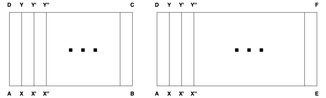
Then,
$$\begin{array}{lclclcl} \Delta(ABCD) & = & \Delta(AXYD) & + & \Delta(XX'Y'Y) & + & \ldots\\ & = & n \cdot \Delta_0, & & & & \end{array}$$and
$$\begin{array}{lclclcl} \Delta(AEFD) & = & \Delta(AXYD) & + & \Delta(XX'Y'Y) & + & \ldots \\ & = & m \cdot \Delta_0 \end{array}$$so that \(\Delta(ABCD)/\Delta(AEFD) = n/m = AB/AE\), as required.
Starting from the early twentieth century, the rigorous proof of the remaining incommensurable case in a school-level exposition typically involves some form of a limit and is based on an implicit or explicit continuity axiom, usually equivalent to Cavaliery principle.
There is, however, a completely elementary, short and elegant proof, that requires no additional assumptions. This proof is used by Legendre (I don't know who is the original author) in his Elements, Éléments de géométrie. Depending on the edition, it is Proposition III in either Book III (p. 100) or Book IV (page 90, some nineteenth-century editions, especially with "additions and modifications by M. A. Blanchet", are butchered beyond recognition, be careful). The proof goes like this:
For incommensurable \(AB\) and \(AE\) consider the ratio \(\Delta(ABCD)/\Delta(AEFD)\). If \(\Delta(ABCD)/\Delta(AEFD) = AB/AE\) we are done. If \(\Delta(ABCD)/\Delta(AEFD)\) is not equal to \(AB/AE\), it is instead equal to \(AB/AO\) and either \(AE < AO\) or \(AE > AO\). Consider the first case (the other one is similar).
The points at the base are in order \(A\), then \(B\), then \(E\), then \(O\).
Divide \(AB\) into \(n\) equal intervals, each shorter that \(EO\). This requires what we now call the Archimedes-Eudoxus axiom and which is implied by Definition IV of Book V:
<λόγον ἔχειν πρὸς ἄλληλα μεγέθη λέγεται, ἃ δύναται πολλαπλασιαζόμενα ἀλλήλων ὑπερέχειν. | Magnitudes are said to have a ratio to one another which can, when multiplied, exceed one another. | Величины имеют отношение между собой, если они взятые кратно могут превзойти друг друга.>
Then continue dividing \(BE\), until we get to a point \(I\) outside of \(BE\), but within \(EO\) (because the interval is shorter than \(EO\)). The points are now in order \(A\), then \(B\), then \(E\), then \(I\), then \(O\).
\(AB\) and \(AI\) are commensurable, so \(\Delta(ABCD)/\Delta(AIKD) = AB/AI\). Also, \(\Delta(ABCD)/\Delta(AEFD) = AB/AO\), so \(\Delta(AIKD)/\Delta(AEFD) = AI/AO\). By construction \(AI < AO\), hence \(\Delta(AIKD) < \Delta(AEFD)\), but \(AEFD\) is a proper part of \(AIKD\), so \(\Delta(AEFD) < \Delta(AIKD)\). Contradiction.
Step back and look at the structure of these two proofs from the modern perspective. Fix the height and let \(\Delta(X)\) be the area of the rectangle with the base of length \(X\). By an assumption that we would call "additivity of measure" \(\Delta(X+Y) = \Delta(X) + \Delta(Y)\), that is, \(\Delta\) is an additive function. A general and easy-to-establish fact (mentioned with remarkable persistency on this blog [Unexpected isomorphism], [The Hunt for Addi(c)tive Monster]) is that any additive function is linear on rationals, that is, \(\Delta(n/m \cdot X) = n/m \cdot \Delta(X)\). This corresponds to the "commensurable" part of the proofs. To complete a proof we need linearity: \(\Delta(X) = X \cdot H\), where \(H = \Delta(1)\). But additive functions are not necessarily linear. To obtain linearity, an additional condition is needed. The traditional proof uses continuity: a continuous (at least at one point) additive function is necessarily linear.
Legendre's proof uses monotonicity: a monotonic additive function is always linear. This is clever, because monotonicity is not an additional assumption: it follows from the already assumed positivity of measure: If \(Y > X\), then \(\Delta(Y) = \Delta(X + (Y - X)) = \Delta(X) + \Delta(Y - X) > \Delta(X)\), as \(\Delta(Y - X) > 0\).
How does the original Euclid's proof look like? (He proves the triangle version, which is similar to rectangles.)

Wait... It is unbelievably short, especially given that the Elements use no notation and spell everything in words and it covers both triangles and parallelograms. It definitely has no separate "commensurable" and "imcommensurable" parts. How is this possible?
The trick is in the definition of equal ratios, Def. V of Book V:
<ἐν τῷ αὐτῷ λόγῳ μεγέθη λέγεται εἶναι πρῶτον πρὸς δεύτερον καὶ τρίτον πρὸς τέταρτον, ὅταν τὰ τοῦ πρώτου καὶ τρίτου ἰσάκις πολλαπλάσια τῶν τοῦ δευτέρου καὶ τετάρτου ἰσάκις πολλαπλασίων καθ᾽ ὁποιονοῦν πολλαπλασιασμὸν ἑκάτερον ἑκατέρου ἢ ἅμα ὑπερέχῃ ἢ ἅμα ἴσα ᾖ ἢ ἅμα ἐλλείπῃ ληφθέντα κατάλληλα.| Magnitudes are said to be in the same ratio, the first to the second and the third to the fourth, when, if any equimultiples whatever are taken of the first and third, and any equimultiples whatever of the second and fourth, the former equimultiples alike exceed, are alike equal to, or alike fall short of, the latter equimultiples respectively taken in corresponding order. | Говорят, что величины находятся в том же отношении: первая ко второй и третья к четвёртой, если равнократные первой и третьей одновременно больше, или одновременно равны, или одновременно меньше равнократных второй и четвёртой каждая каждой при какой бы то ни было кратности, если взять их в соответственном порядке>
In modern notation this means that
$$\Delta_1 / \Delta_2 = b_1 / b_2 \equiv (\forall n\in\mathbb{N}) (\forall m\in\mathbb{N}) (n\cdot\Delta_1 \gtreqqless m\cdot\Delta_2 = n\cdot b_1 \gtreqqless m\cdot b_2),$$where \(\gtreqqless\) is "FORTRAN 3-way comparison operator" (aka C++ spaceship operator):
$$X \gtreqqless Y = \begin{cases} -1, & X < Y\\ 0, & X = Y\\ +1, & X > Y \end{cases}$$This looks like a rather artificial definition of ratio equality, but with it the proof of Proposition I and many other proofs in Books V and VI, become straightforward or even forced.
The approach of selecting the definitions to streamline the proofs is characteristic of abstract twentieth-century mathematics and it is amazing to see it in full force in the earliest mathematical text we have.
I'll conclude with the promised anecdote (unfortunately, I do not remember the source). An acquaintance of Newton having met him in the Cambridge library and found, on inquiry, that Newton is reading the Elements, remarked something to the effect of "But Sir Isaac, haven't your methods superseded and obsoleted Euclid?". This is one of the two recorded cases when Newton laughed.
[0]
Let's find a sum
$$\sum_{n=1}^\infty {1\over{n(n+2)}}$$There is a well-know standard way, that I managed to recall eventually. Given that
$${1 \over n(n+2)} = {1 \over 2}\cdot \left({1\over n} - {1\over n+2}\right)$$the sum can be re-written as
$$\sum_{n=1}^\infty {1\over{n(n+2)}} = \sum_{n=1}^\infty {1 \over 2}\left({1\over n} - {1\over n+2}\right) = {1\over 2}\left({1\over 1} - {1\over 3} + {1\over 2} - {1\over 4} + {1\over 3} - {1\over 5} + {1\over 4} - {1\over 6} \cdots\right)$$with almost all terms canceling each other, leaving
$$\sum_{n=1}^\infty {1\over{n(n+2)}} = {1\over 2}\left(1 + {1\over 2}\right) = {3\over 4}$$While this is easy to check, very little help is given on understanding how to arrive to the solution in the first place. Indeed, the first (and crucial) step is a rabbit pulled sans motif out of a conjurer hat. The solution, fortunately, can be found in a more systematic fashion, by a relatively generic method. Enter generating functions.
First, introduce a function
$$f(t) = \sum_{n=1}^\infty {t^{n + 1}\over n}$$The series on the right converge absolutely when \(|t| < 1\), so one can define
$$g(t) = \int f(t) dt = \int \sum_{n=1}^\infty {t^{n + 1}\over n} = \sum_{n=1}^\infty \int {t^{n + 1}\over n} = \sum_{n=1}^\infty {t^{n + 2}\over {n(n+2)}} + C$$with the sum in question being
$$\sum_{n=1}^\infty {1\over{n(n+2)}} = g(1) - C = g(1) - g(0)$$Definition of the \(g\) function follows immediately from the form of the original sum, and there is a limited set of operations (integration, differentiation, etc.) applicable to \(g\) to produce \(f\).
The rest is more or less automatic. Note that
$$- ln(1 - t) = t + {t^2\over 2} + {t^3\over 3} + \cdots$$so that
$$f(t) = t^2 + {t^3\over 2} + {t^4\over 3} + \cdots = - t \cdot ln(1-t)$$therefore
$$g(t) = - \int t \cdot ln(1-t) dt = \cdots = {1\over 4} (1 - t)^2 - {1\over 2} (1 - t)^2 ln(1 - t) + (1 - t) ln(1 - t) + t + C$$where the integral is standard. Now,
$$g(1) - g(0) = 1 - {1\over 4} = {3\over 4}$$Voilà!
And just to check that things are not too far askew, a sub-exercise in pointless programming:
scala> (1 to 10000).map(x => 1.0/(x*(x+2))).reduceLeft(_+_)
res0: Double = 0.749900014997506
PS: of course this post is an exercise in tex2img usage.
PPS: Ed. 2022: tex2img is gone, switch to mathjax.
ext3 htree code in Linux kernel implements peculiar version of balanced tree used to efficiently handle large directories.
htree directory consists of block sized nodes. Some of them (leaf nodes) contain directory entries in the same format as ext2. Other nodes contain index: they are filled with hashes and pointers to other nodes.
When new file is created in a directory, a directory entry is inserted in one of leaf nodes. When leaf node has not enough space for new entry, new node is appended to the tree, and part of directory entries is moved there. This process is known as a split. Pointer to new node is then inserted into some index node, and new node can overflow at this point, causing another split and so on.
If splits occur whole way up to the root of the tree, new root has to be added (tree grows).
It's obvious that in the worst case (extremely rare in practice) insertion of a new entry may require a new block on each tree level, plus new root, right? Now, looking at the ext3_dx_add_entry() function we see something strange:
                 } else {
                         dxtrace(printk("Creating second level index...\n"));
                         memcpy((char *) entries2, (char *) entries,
                                icount * sizeof(struct dx_entry));
                         dx_set_limit(entries2, dx_node_limit(dir));

                         /* Set up root */
                         dx_set_count(entries, 1);
                         dx_set_block(entries + 0, newblock);
                         ((struct dx_root *) frames[0].bh->b_data)->info.indirect_levels = 1;

                         /* Add new access path frame */
                         frame = frames + 1;
                         frame->at = at = at - entries + entries2;
                         frame->entries = entries = entries2;
                         frame->bh = bh2;
                         err = ext3_journal_get_write_access(handle,
                                                              frame->bh);
                         if (err)
                                 goto journal_error;
                 }
At this moment entries points to the already existing full node and entries2 to the newly created one. As one can see, contents of entries is shifted into entries2, and entries is declared to be new root of the tree. So now tree has a root node with a single pointer to the index node that... still has not enough free space (remember entries2 got everything entries had). Omitted code that follows proceeds with splitting leaf node, assuming that its parent has enough space to insert a pointer to the new leaf. So how this is supposed to work? Or, does this work at all? That's tricky part and the curious reader is invited to try to infer what's going on without looking at the rest of this post.
The answer is simple: by ext3 htree design, capacity of the root node is smaller than that of non-root index one. This is a byproduct of binary compatibility between htree and old ext2 format: root node is always the first block in the directory and it always contains dot and dotdot directory entries. As a result, when contents of old root is copied into new node, that node ends up having enough space for two additional entries.
This is obviously one of the worst hacks and least documented at that. Shame.
Thanks to Alex Tomas for clearing this mystery for me. As he says: "Htree code is simple to understand: it only takes to tune yourself to Daniel Phillips brain-waves frequency".
"feminism means freedom, it means the right to be ... incoherent", p. 71
Let me state outright, that I won't be able to provide a critique of the cogent rational argument that forms the core of Ms. Olufemi's book, for the simple fact that even the most diligent search will not find an argument of that sort there.
I am going to prove with ample internal and external evidence, that the book does not present an articulated argument for anything. That it is little more than a haphazard collection of claims, that are not only not supported by evidence, but do not even form a consistent sequence.
All references are to the paperback 2020 edition.
Preamble
The most striking feature of the book before us is that it is difficult to find a way to approach it. A sociological study and a political pamphlet still have something in common: they have a goal. The goal is to convince the reader. The methods of convincing can be quite different, involve data and logic and authority. But in any case, something is needed. As you start reading Feminism Interrupted you are bound to find that this something is hidden very well. Indeed, as I just counted, one of the first sections Who's the boss has as many claims as it has sentences (some claims are in the form of rhetorical questions). There, as you see, was no space left for any form of supporting argumentation. Because it is not immediately obvious how to analyse a text with such a (non-)structure, let me start the same way as Ms. Olufemi starts in Introduction and just read along, jotting down notes and impressions, gradually finding our way through the book, forming a conception of the whole.
The following is a numbered list of places in the book that made me sigh or laugh. They are classified as: E (not supported by Evidence), C (Contradiction with itself or an earlier claim) and I (Incoherence). These classes are necessarily arbitrary and overlapping. I will also provide a commentary about some common themes and undercurrents running through the book.
One may object that this is too pedantic a way to review a book. Well, maybe it is, but this is the only way I know to lay ground for justifiable conclusions, with which my review will be concluded.
Notes on the text
1.E, p. 4: "neo-liberalism refers to the imposition of cultural and economic policies and practices by NGOs and governments in the last three to four decades that have resulted in the extraction and redistribution of public resources from the working class upwards" — this of course has very little to do with the definition of Neo-liberalism. Trivial as it is, this sentence introduces one of the most interesting and unexpected themes that will resurface again and again: Ms. Olufemi, a self-anointed radical feminist from the extreme left of the political spectrum, in many respects is virtually indistinguishable from her brethren on the opposite side. Insidious "NGOs" machinating together with governments against common people are the staple imagery of the far-right.
2.C, p. 5: "... that feminism has a purpose beyond just highlighting the ways women are 'discriminated' against... It taught me that feminism's task is to remedy the consequences of gendered oppression through organising... For me, 'justice work' involves reimagining the world we live in and working towards a liberated future for all... We refuse to remain silent about how our lives are limited by heterosexist, racist, capitalist patriarchy. We invest in a political education that seeks above all, to make injustice impossible to ignore." — With a characteristic ease, that we will appreciate to enjoy, Ms. Olufemi tells us that feminism is not words, and in the very next sentence, supports this by her refusal to remain silent.
3.C, p. 7: "Pop culture and mainstream narratives can democratise feminist theory, remove it from the realm of the academic and shine a light on important grassroots struggle, reminding us that feminism belongs to no one." — Right after being schooled on how the iron fist of capitalist patriarchy controls every aspect of society, we suddenly learn that the capitalist society media welcomes the revolution.
4.C, p. 8: This is the first time that Ms. Olufemi has decided to grace us with a cited source (an article from Sp!ked, 2018). The reference is in the form of a footnote, and the footnote is a 70-character URL. That is what almost all her references and footnotes look like. A particularly gorgeous URL is in footnote 3 on p. 53: it's 173 characters, of which the last 70 are unreadable gibberish. Am I supposed to retype this character-by-character on my phone? Or the references are for ornamentation only? In any case, it seems Ms. Olufemi either cannot hide her extreme contempt for the readers, or spent her life among people with an unusual amount of leisure.
5.E, p. 15: "When black feminists ... organised in the UK ... [t]hey were working towards collective improvement in material conditions... For example..." — The examples provided are: Grunwick strike by South Asian women and an Indian lady, Jayaben Desai. Right in the next sentence after that, Ms. Olufemi concludes: "There is a long history of black women ... mounting organised and strategic campaigning and lobbying efforts". Again as in 2.C, she is completely unabated by the fact that the best examples of black feminist activities that she is able to furnish, have nothing to do with black feminists.
6.E. p. 23: "Critical feminism argues that state sexism has not lessened [for the last 50 years]". Evidence: "MPs in parliament hide the very insidious ways that the state continues to enable male dominance ... " — tension rises! — "the Conservative government introduced their plans to pass a Domestic Violence Bill with the intention of increasing the number of convictions for perpetrators of abuse... " — which looks good on the surface, but of course — "it is simply another example of the way the state plays on our anxieties about women's oppression to disguise the enactment of policies that trap women in subordinate positions." — Finally, we are about to learn how exactly the governments (and NGOs, remember!) keep women subjugated for the last 50 years, we are agog with curiosity! — "Research from the Prison Reform Trust has found an increase in the number of survivors being arrested" (p. 24) — And then... And then there is nothing. How does this prove that things are not better than 50 years ago? Just follow Mr. Olufemi example, and completely expunge from your mind everything that you claimed more than five sentences and seconds ago.
7.C, p. 26. "But this figure does not tell the whole story. The impact of these cuts is felt particularly by low-income black women and women of colour." — Another constant motif of the book is that Ms. Olufemi alternately blames the state for violence and overreach, only to immediately request expansion of paternalistic services and welfare.
8.C, p. 27: "If a woman must disclose ... that she has been raped ... her dignity, agency and power over personal information is compromised." — In a sudden turn of events our feminist seems to argue that it would be preferable for rape survivors to stay silent.
9.E, p. 28: When she does provide any sort of supporting evidence, it feels better that she wouldn't: "We know that thousands of disabled people have died as a direct result of government negligence surrounding Personal Independence Payments ...\((^9)\)" — The footnote is nothing but a 100 character URL, that I patiently typed in, only to be greeted with 404. According to webarchive.org, the referred-to page never existed. Ultimately, after many false starts (whose details I shall spare you), I found the document at a completely different web-site:
https://questions-statements.parliament.uk/written-questions/detail/2018-12-19/203817
Imagine my (lack of) surprise, when it turned out that government "negligence" is neither mentioned nor in any way implied or imputed—Ms. Olufemi simply fabricated the whole story.
10.I, p.29: "[In Yarl's Wood IRC] they are locked in, unable to leave and subjected to surveillance by outsourced security guards. Tucked away in Bedford outside of the public consciousness, it's hard to think of a more potent example of state violence." — Judgment of anybody who, in the world of wars, continuous genocides and slaughter of human beings, maintains that the worst example of state violence is the sufferings of the women, who fled their ruined countries to the relative safety of the UK, must be thoroughly questioned. The second quoted sentence is also indefensible grammatically.
11.E, p. 30: In support of her claim that the state violently oppresses black women, Ms. Olufemi provides stories of 3 black women, that died in police custody over the course of... 50 years. "they reveal a pattern" — she confidently concludes. No, they don't. Statistical data would, but they do not support Ms. Olufemi's thesis. She then proceeds to lament "a dystopian nightmare for the undocumented migrants" — conveniently forgetting that these people tried as hard as they could to move to the dystopian UK and none of them hurried back. The section the quote is from is called State Killings — the 3 examples provided are somehow put in the same rubric as the doings of Pol-Pot and Mao.
12.E, p. 31: "If black women die disproportionately at the hands of the police, historically and in the present moment" — and then she proceeds on the assumption that they do, without providing any evidence. Immediately available public data (from INQUEST and IOPC reports), clearly refute the premise.
13.C, p. 32: "This refusal to participate [in capitalism] takes many forms: feminist activists are finding new and creative ways to oppose austerity." — Ms. Olufemi's personal creative way to refuse to participate in the capitalist economy is to copyright a book, publish it with a publishing corporation (a capitalist enterprise, mind you) and then collect the royalties.
14.E., p. 33: "Sisters Uncut has put domestic and sexual violence on the national agenda" — Ms. Olufemi's desire to prop her friends is laudable, but it does not eliminate the need to provide evidence.
15.I., p.33: "When I ask Sandy where the idea to create Sisters came from, she tells me" — Who's Sandy? No Sandy was mentioned before. A certain Sandy Stone, the author of A Posttranssexual Manifesto appears 30 pages later, but it is unlikely she is meant here. The simple present tense of the sentence uncannily reminds of the way children talk about their imaginary friends.
16.C., p. 36: "So that just ... – Shulamith Firestone" — Oops, Ms. Olufemi approvingly quotes S. Firestone — a central figure in the so much derided second-wave liberal feminism.
17.C, p. 38: Trying to tie 'social reproduction' to race, Ms. Olufemi notices: "Wealthy white women have always been able to exercise greater agency over their reproductive capacity because they can afford private healthcare and specialist medical advice", omitting to mention that so have wealthy black women too. The difference, as she herself emphasised with the "because" part, is in wealth not race. Mr. Olufemi then proceeds to build far-reaching conclusions from this rather trivial error.
18.E, p. 39: Being a radical revolutionary, Ms. Olufemi is not afraid to cast aspersions on defenceless dead women: "Margaret Sanger, reproductive rights advocate responsible for the first birth control-clinic in the United States was a vocal eugenicist" — the consensus in the literature is that M. Sanger was not a eugenist or racist in any shape of form. See
Roberts, Dorothy (1998). Killing the Black Body: Race, Reproduction, and the Meaning of Liberty. Knopf Doubleday. ISBN 9780679758693. LCCN 97002383, p.77--78
Gordon, Linda (2002). The Moral Property of Women: A History of Birth Control Politics in America. University of Illinois Press. ISBN 9780252027642.
Valenza, Charles (1985). "Was Margaret Sanger a Racist?". Family Planning Perspectives. 17 (1). Guttmacher Institute: 44–46. doi:10.2307/2135230. JSTOR 2135230. PMID 3884362
Ms. Olufemi's source? Angela Davis. At this point, let me make an aside. Ms Olufemi treats Angela Davis as a kind of mother figure and a hero: she quotes her left and right, and puts her on the blurb of the back cover. Angela Davis, in the meantime, is a KGB stooge, a "useful idiot" in an apt expression of Lenin. That beacon of freedom-fighting unashamedly praised and was on the pay of the Soviet communist regime that, as was very well-known at the time, organised the extermination of tens of millions of people.
19.C, p. 41: Suddenly Ms. Olufemi lashes out against contraceptives, linking them to... eugenic: "eugenics has shaped our notion of family ... the racist logic of 'population control' that birthed the desire for contraceptives" — in this place again, it's difficult to tell her from far-right and religious fundamentalists.
20.C, p. 44: "nobody understands the stakes around the right to access abortion and reproductive justice more than working class women" — That looks like a good point to discuss Ms. Olufemi's background. Far from being qualified to understand the "stakes", she comes from what definitely does not look like a working class: after graduating from a privileged grammar school, she was immediately forced by the oppressive patriarchal society to study at Cambridge. Her PhD. research was sponsored (via TECHNE AHRC) by the very same government that she so mercilessly scrutinises in the present opus.
21.E, p. 44: "Ireland is coded 'white', and 'Irish woman' means only those who fall under that coding" — neither of these claims is supported. Fortunately they are, as usual, in no way used in the following, because Ms Olufemi quickly switches to other, equally unsupported, claims.
22.E, p. 47: "English MPs voted ... to change Northern Ireland's abortion law .... This means that Abortion in Northern Ireland has only recently been decriminalised, the possibility of persecution has been lifted from those administering and undergoing abortions." — (Capitalisation as in the original.) There were no "underground" abortions in N. Ireland, because free abortions were available in England, a few hours away on a ferry.
23.E, p. 47: "The tendency to consider the UK a progressive environment for reproductive justice sorely underestimates the number of people, who despite the change in law may still have no recourse to abortion services" — Well, then tell us.
24.E, p. 48: "Winning radically would mean ... a world without work" — That's refreshingly honest, even though Marx won't approve of such blatant revisionism.
25.E, p. 50: "throughout history, to be 'female' has often meant death, mutilation and oppression" — this unsupported claim is clearly wrong. Throughout history, most victims of violence by a large margin were and are men. Most people killed in the wars are men. Most people dying a violent death are men. Most people in prisons and mental institutions are men. More than 90% of work-related deaths happen to men.
26.I, p. 50: "If there are only two categories, it is easier for us to organise the world and attach feelings, emotions and ways of being to each one." — If it were so, then all categories would have been binary: there would have been 2 nations, 2 fashion styles, etc.
27.C, p. 50 Ms. Olufemi continues to argue that gender is fluid and a person can change it at will. Her arguments: "there is no way to adequately describe what gender is. Every definition does a disservice to the shifting, multiple and complex set of power relations that come to shape a person's gender." — It would be interesting to trace her train of thought if "gender" were replaced with "race" in this sentence. As race is much more of a social construct and less rooted in biology, surely Ms. Olufemi would agree that we should welcome when a "racially dysphoric" white person claims to be black. Unfortunately that would uproot her basic tenet about the exclusivity of black women's experience and its central role in the formation of radical feminism.
28.C, p. 52: "If one group of people consistently behave, speak, move, present themselves in one way and another in the 'opposite' way, we reaffirm the idea that there is actually an inherent difference between those two groups when no such difference exists." — I guess the groups Ms. Olufemi has in mind are males and females. Or maybe whites and blacks?
29.C, p. 52: "Many intersex infants ... have surgery to 'correct' their genitalia without their consent." — That's an interesting notion. Should we abstain from, for example, fixing broken bones of small children, until such time as they would be mature enough to consent?
30.E, p. 53: "Many women are physically stronger than men; many men are physically weaker than women. These are not exceptions that defy a rule; there simply is no rule." — This betrays an utter ignorance of statistics and data. Normal distribution of strength (as measured, for example, by grip tests) in a population with different means for males and females is among the most reliably established anthropometrical facts.
31.E, p. 54: "To argue that there is a clear difference between sex and gender serves to solidify the idea that biological sex, prior to human beings inventing it and naming its tenants, exists." — here again Ms. Olufemi joins far-right and religious fundamentalists in her anti-science stance and denial of the evolutionary origin of mechanisms of sexual reproduction. The objective existence of biological sex, manifested in morphological, physiological and behavioural differences (sexual dimorphism) is attested beyond the slightest doubt across the entire animal kingdom.
32.E, p.68: "It is the public rejoicing at 19-year-old Shamima Begum being stripped of her citizenship" — Ms. Olufemi chose as her example of Islamophobia a girl who joined ISIS, and became there an enforcer that threatened other women with death lest they comply with ISIS rules, stripped suicide vests into their clothes and ended up burying all her 3 children in this non-secular utopia.
33.E, p. 71: "Muslim women are the most economically disenfranchised group in the country." — this simple claim is simply wrong. According to the UK Office for National Statistics, the most economically disenfranchised group in the UK are (as expected) refugees and asylum seekers, followed (unfortunately for Ms. Olufemi) by white workers in "post-industrial" (read: de-industrialised) communities.
34.C, p. 74: "A staunchly secular way of thinking about our lives and bodies limits Muslim women's ability to understand themselves" — Ms. Olufemi sympathy for organised monotheistic religions and her distrust in the secular society is rather unexpected. It is not clear how to reconcile her idea that to better understand themselves women should abandon secularism and return to the church or mosque with the feminist dogma.
35.I, p. 76: "creation of a public outcry about 'Asian Grooming Gangs.'" — It's sad that a feminist can scary-quote and dismiss one of the most horrible cases of mass abuse of women. A sacrifice of the suffering of more than a thousand girls to make a vindictive political point does not paint Ms. Olufemi as a good human being.
36.I, p. 86: "Art is a tool for feminist propaganda" — Unfortunately Ms. Olufemi forgot that this chapter is called Art for Art's Sake and its main thesis is that art of not a tool of anything. Notice also how she repeats Stalin and Goebbels almost verbatim.
37.C, p. 88: "Poor women do not get to make art: the fact that Saye's work could be displayed in one of the most prestigious arenas in the world ... calls us to wake up to the cruelty of inequity. " — This is probably one of the most impressive examples of Ms. Olufemi's ability to forget the beginning of a sentence (that she wrote!) by the time she gets to its middle — she demonstrates that poor women cannot make art by an example of a poor woman whose art became fashionable and famous. But then she easily outdoes herself! By the time we get to the end of the sentence, she forgets what was in the middle (or otherwise she thinks that being displayed at a Venice Biennale is unusually cruel).
38.C, p. 89: "Momtaza Mehri, essayist, researcher and former Poet Laureate for young people, tells me. " — Ms. Olufemi continues to give proof of art being unavailable to poor women by providing another example: of a poor woman who was a Poet Laureate.
39.I, p. 110: "The idea that justice is served when criminals go to prison is relatively new. ... Ironically, prisons were introduced in order to make punishment more 'humane'." — Unironically, this is one of the most blatantly ignorant statements to grace the printing press lately. Prisons, as known to anybody with even superficial knowledge of history, existed as long as states did. There are some echoes of Foucault in that sentence, but poorly read or remembered, because his conclusion was the opposite.
40.E, p. 123: "In July 2019, Cancer Research UK, fundraising partners with dieting organisation Slimming World, launched a multi-million pound campaign using defunct scientific indicators to claim that obesity was the second leading cause of cancer." — This is outright dangerous. Spreading falsehoods to the vulnerable people in the risk groups is extremely irresponsible. Large‑scale cohort studies show that higher body mass index (BMI) and excess adiposity correlate with increased incidence and worse outcomes for multiple cancer types. These data form the backbone of public‑health recommendations promoting weight management:
Renehan AG, Tyson M, Egger M, Heller RF, Zwahlen M. "Body-mass index and incidence of cancer: a systematic review and meta-analysis of prospective observational studies." The Lancet, 371(9612), 569-578 (2008).
Bhaskaran K, Douglas I, Forbes H, dos-Santos-Silva I, Leon DA, Smeeth L. "Body-mass index and risk of 22 specific cancers: a population-based cohort study of 5·24 million UK adults." The Lancet, 384(9945), 755-765 (2014).
41.I, p. 124: "There is no clearer manifestation of neo-liberalism than in our attitudes towards bodies." — this, in the words of Pauli "is not even wrong", whatever "attitudes toward bodies" means, they are not the clearest manifestation of neo-liberalism.
42.C, p. 125: "the myth that fatness means ill health" — Again, Ms Olufemi would be home with far-right conspiracy theorists. Excess adipose tissue (body fat) is strongly linked to a variety of health problems, including hypertension, insulin resistance, type 2 diabetes, cardiovascular disease, sleep apnea, and certain cancers. Medical researchers generally treat obesity as a risk factor that actively contributes to many of these conditions.
43.I, p. 126: "Nearly half of single parents in the UK – working or unemployed – live in relative poverty." — That's because relative poverty is defined by the UK statistical agencies as "being poorer than half of the population".
At this point your humble Scheherazade broke off in exhaustion.
Conclusions
"we need to remove the shame in the way we talk about acceptable forms of killing" — p. 48
I hope my notes demonstrated that even the most lenient and indulgent reader would quickly conclude that Feminism Interrupted is balderdash. That would be, however, too trivial a conclusion. Everything has a purpose and Ms. Olufemi book can find one with our help. As far as I can see, the purpose is to realise that even though incoherent and rambling, the text has a texture, some recurrent images appear again and again:
1. Ms Olufemi continuously laments the exploitation, poverty and oppression of women in the UK. Well, as everything in human condition, exploitation is relative. Ms. Olufemi enjoys the life of comfort, privilege and ease unimaginable to anyone outside of the scopes of the "developed" (i.e., capitalist) world or the last hundred years. She imagines a utopia of a stateless society free of "exploitation", but there is no indication that this eschaton is possible. It is not even a practical possibility that is questionable, but logical: is her image free of internal contradictions? All attempts to realise this millenialist dream, from Bogomils to Soviet and Chinese communists, are remembered for little besides industrial scale murder they invariably resulted in.
2. Ms. Olufemi's feelings toward organised religion are clearly ambiguous. On one hand, she presumably understands that organised religion is the core institution of patriarchy that maintains and perpetuates values and structures that she finds so odious. On the other hand, she obviously cannot stop expressing her admiration of the austere faith of Mohammed, comparing it favourably with the decadent secular societies of the West.
3. Ms. Olufemi cannot decide whether she wants to abolish the state or expand it tremendously. Often in the course of the same period she registers her conviction that the state is evil and should be abolished, only to proceed to point out how unjust it is that the state does not sufficiently help the dispossessed and to request enlargement of welfare.
4. As was noted on many occasions, many of Ms. Olufemi's positions echo ones of far-right conspirologists. Her distrust of science and NGOs makes one reconsider the "horseshoe theory" favourably.
[Updated: 2005.07.24]
A scary thing happened to me: my first thought, while looking at linux-2.6.5-7.151/lib/vsprintf.c
if (*fmt == 'h' || *fmt == 'l' || *fmt == 'L' ||
    *fmt == 'Z' || *fmt == 'z') {
    qualifier = *fmt;
    fmt++;
}
was something like Hmm... I should be careful about that master lich here.... I should throttle down.
Yes, this turned out to be a gcc bug
I hit what more and more looks like a bug in the standard Ubuntu 24 gcc version. Here is a minimal reproducer that I with great pain extracted from 12KLOC sources:
struct foo {
        int   seq;
        void *data;
};

struct bar {
        struct foo rung[1];
};

static int used;

static char ll(const struct foo *n) {
        return *(char *)n->data;
}

int main(int argc, char **argv) {
        struct bar p = {};
        int result = 0;
        used = 0;
        __asm__ __volatile__("": : :"memory");
        for (int i = 0; i <= used && result == 0; ++i) {
                struct foo *r = &p.rung[i];
                __attribute__((assume(i <= 0 || ll(r) + 1 == ll(r - 1))));
                if (!(r->seq == 0 && (i <= 0 || ll(r) + 1 == ll(r - 1)))) {
                        result = -1;
                }
        }
        return 0;
}
Compile as gcc -O1 gcc-13-bug.c, it crashes with SIGSEGV. Note that because the loop iterates only once, i == 0 in the body of the loop, so ll(r) should not be called. Yet, ll(r) and ll(r-1) are both called.
The reproducer is minimal in the sense that it is locally optimal: any small random change eliminates the effect. For example,
Move used = 0 over the asm-barrier (or simply remove the barrier).
Remove result == 0 from the loop guard.
Replace struct bar p = {} with struct foo[1] p = {} mutatis mutandis. This one is especially surprising.
Quite some time ago (in the previous century), gcc greeted me with the following self-explanatory message (My feelings toward C++ only increased since then.):
src/algorithms/parse/GrammarNode.cpp:114: `((new QR::ObjectWrapper(((new QR::Concatenation("barNo",
new QR::List(2, ((new QR::ObjectWrapper(((new QR::Terminal("bar", new QR::String("keyword_bar")) !=
0) ? new QR::Terminal("bar", new QR::String("keyword_bar"))->QR::Terminal::_vb.Q22QR11GrammarNode->
QR::GrammarNode::_vb.Q22QR6Object->QR::Object::_vb.Q22QR3Top : 0)) != 0) ? new QR::ObjectWrapper(((
new QR::Terminal("bar", new QR::String("keyword_bar")) != 0) ? new QR::Terminal("bar", new QR::Stri
ng("keyword_bar"))->QR::Terminal::_vb.Q22QR11GrammarNode->QR::GrammarNode::_vb.Q22QR6Object->QR::Ob
ject::_vb.Q22QR3Top : 0))->QR::ObjectWrapper::_vb.Q22QR6Object->QR::Object::_vb.Q22QR3Top : 0), ((n
ew QR::ObjectWrapper(((new QR::Terminal("< >", new QR::String("Whitespace")) != 0) ? new QR::Termin
al("< >", new QR::String("Whitespace"))->QR::Terminal::_vb.Q22QR11GrammarNode->QR::GrammarNode::_vb
.Q22QR6Object->QR::Object::_vb.Q22QR3Top : 0)) != 0) ? new QR::ObjectWrapper(((new QR::Terminal("<
", new QR::String("Whitespace")) != 0) ? new QR::Terminal("< >", new QR::String("Whitespace"))->QR
::Terminal::_vb.Q22QR11GrammarNode->QR::GrammarNode::_vb.Q22QR6Object->QR::Object::_vb.Q22QR3Top :
0))->QR::ObjectWrapper::_vb.Q22QR6Object->QR::Object::_vb.Q22QR3Top : 0), ((new QR::ObjectWrapper((
(new QR::Terminal("no", new QR::String("NumericLiteral")) != 0) ? new QR::Terminal("no", new QR::St
ring("NumericLiteral"))->QR::Terminal::_vb.Q22QR11GrammarNode->QR::GrammarNode::_vb.Q22QR6Object->Q
R::Object::_vb.Q22QR3Top : 0)) != 0) ? new QR::ObjectWrapper(((new QR::Terminal("no", new QR::Strin
g("NumericLiteral")) != 0) ? new QR::Terminal("no", new QR::String("NumericLiteral"))->QR::Terminal
::_vb.Q22QR11GrammarNode->QR::GrammarNode::_vb.Q22QR6Object->QR::Object::_vb.Q22QR3Top : 0))->QR::O
bjectWrapper::_vb.Q22QR6Object->QR::Object::_vb.Q22QR3Top : 0), 0)) != 0) ? new QR::Concatenation("
barNo", new QR::List(2, ((new QR::ObjectWrapper(((new QR::Terminal("bar", new QR::String("keyword_b
ar")) != 0) ? new QR::Terminal("bar", new QR::String("keyword_bar"))->QR::Terminal::_vb.Q22QR11Gram
marNode->QR::GrammarNode::_vb.Q22QR6Object->QR::Object::_vb.Q22QR3Top : 0)) != 0) ? new QR::ObjectW
rapper(((new QR::Terminal("bar", new QR::String("keyword_bar")) != 0) ? new QR::Terminal("bar", new
QR::String("keyword_bar"))->QR::Terminal::_vb.Q22QR11GrammarNode->QR::GrammarNode::_vb.Q22QR6Object
->QR::Object::_vb.Q22QR3Top : 0))->QR::ObjectWrapper::_vb.Q22QR6Object->QR::Object::_vb.Q22QR3Top :
0), ((new QR::ObjectWrapper(((new QR::Terminal("< >", new QR::String("Whitespace")) != 0) ? new QR:
:Terminal("< >", new QR::String("Whitespace"))->QR::Terminal::_vb.Q22QR11GrammarNode->QR::GrammarNo
de::_vb.Q22QR6Object->QR::Object::_vb.Q22QR3Top : 0)) != 0) ? new QR::ObjectWrapper(((new QR::Termi
nal("< >", new QR::String("Whitespace")) != 0) ? new QR::Terminal("< >", new QR::String("Whitespace
"))->QR::Terminal::_vb.Q22QR11GrammarNode->QR::GrammarNode::_vb.Q22QR6Object->QR::Object::_vb.Q22QR
3Top : 0))->QR::ObjectWrapper::_vb.Q22QR6Object->QR::Object::_vb.Q22QR3Top : 0), ((new QR::ObjectWr
apper(((new QR::Terminal("no", new QR::String("NumericLiteral")) != 0) ? new QR::Terminal("no", new
QR::String("NumericLiteral"))->QR::Terminal::_vb.Q22QR11GrammarNode->QR::GrammarNode::_vb.Q22QR6Obj
ect->QR::Object::_vb.Q22QR3Top : 0)) != 0) ? new QR::ObjectWrapper(((new QR::Terminal("no", new QR:
:String("NumericLiteral")) != 0) ? new QR::Terminal("no", new QR::String("NumericLiteral"))->QR::Te
rminal::_vb.Q22QR11GrammarNode->QR::GrammarNode::_vb.Q22QR6Object->QR::Object::_vb.Q22QR3Top : 0))-
QR::ObjectWrapper::_vb.Q22QR6Object->QR::Object::_vb.Q22QR3Top : 0), 0))->QR::GrammarNode::_vb.Q22
QR6Object->QR::Object::_vb.Q22QR3Top : 0)) != 0) ? new QR::ObjectWrapper(((new QR::Concatenation("b
arNo", new QR::List(2, ((new QR::ObjectWrapper(((new QR::Terminal("bar", new QR::String("keyword_ba
r")) != 0) ? new QR::Terminal("bar", new QR::String("keyword_bar"))->QR::Terminal::_vb.Q22QR11Gramm
arNode->QR::GrammarNode::_vb.Q22QR6Object->QR::Object::_vb.Q22QR3Top : 0)) != 0) ? new QR::ObjectWr
apper(((new QR::Terminal("bar", new QR::String("keyword_bar")) != 0) ? new QR::Terminal("bar", new
QR::String("keyword_bar"))->QR::Terminal::_vb.Q22QR11GrammarNode->QR::GrammarNode::_vb.Q22QR6Object
->QR::Object::_vb.Q22QR3Top : 0))->QR::ObjectWrapper::_vb.Q22QR6Object->QR::Object::_vb.Q22QR3Top :
0), ((new QR::ObjectWrapper(((new QR::Terminal("< >", new QR::String("Whitespace")) != 0) ? new QR:
:Terminal("< >", new QR::String("Whitespace"))->QR::Terminal::_vb.Q22QR11GrammarNode->QR::GrammarNo
de::_vb.Q22QR6Object->QR::Object::_vb.Q22QR3Top : 0)) != 0) ? new QR::ObjectWrapper(((new QR::Termi
nal("< >", new QR::String("Whitespace")) != 0) ? new QR::Terminal("< >", new QR::String("Whitespace
"))->QR::Terminal::_vb.Q22QR11GrammarNode->QR::GrammarNode::_vb.Q22QR6Object->QR::Object::_vb.Q22QR
3Top : 0))->QR::ObjectWrapper::_vb.Q22QR6Object->QR::Object::_vb.Q22QR3Top : 0), ((new QR::ObjectWr
apper(((new QR::Terminal("no", new QR::String("NumericLiteral")) != 0) ? new QR::Terminal("no", new
QR::String("NumericLiteral"))->QR::Terminal::_vb.Q22QR11GrammarNode->QR::GrammarNode::_vb.Q22QR6Obj
ect->QR::Object::_vb.Q22QR3Top : 0)) != 0) ? new QR::ObjectWrapper(((new QR::Terminal("no", new QR:
:String("NumericLiteral")) != 0) ? new QR::Terminal("no", new QR::String("NumericLiteral"))->QR::Te
rminal::_vb.Q22QR11GrammarNode->QR::GrammarNode::_vb.Q22QR6Object->QR::Object::_vb.Q22QR3Top : 0))-
QR::ObjectWrapper::_vb.Q22QR6Object->QR::Object::_vb.Q22QR3Top : 0), 0)) != 0) ? new QR::Concatena
tion("barNo", new QR::List(2, ((new QR::ObjectWrapper(((new QR::Terminal("bar", new QR::String("key
word_bar")) != 0) ? new QR::Terminal("bar", new QR::String("keyword_bar"))->QR::Terminal::_vb.Q22QR
11GrammarNode->QR::GrammarNode::_vb.Q22QR6Object->QR::Object::_vb.Q22QR3Top : 0)) != 0) ? new QR::O
bjectWrapper(((new QR::Terminal("bar", new QR::String("keyword_bar")) != 0) ? new QR::Terminal("bar
", new QR::String("keyword_bar"))->QR::Terminal::_vb.Q22QR11GrammarNode->QR::GrammarNode::_vb.Q22QR
6Object->QR::Object::_vb.Q22QR3Top : 0))->QR::ObjectWrapper::_vb.Q22QR6Object->QR::Object::_vb.Q22Q
R3Top : 0), ((new QR::ObjectWrapper(((new QR::Terminal("< >", new QR::String("Whitespace")) != 0) ?
new QR::Terminal("< >", new QR::String("Whitespace"))->QR::Terminal::_vb.Q22QR11GrammarNode->QR::Gr
ammarNode::_vb.Q22QR6Object->QR::Object::_vb.Q22QR3Top : 0)) != 0) ? new QR::ObjectWrapper(((new QR
::Terminal("< >", new QR::String("Whitespace")) != 0) ? new QR::Terminal("< >", new QR::String("Whi
tespace"))->QR::Terminal::_vb.Q22QR11GrammarNode->QR::GrammarNode::_vb.Q22QR6Object->QR::Object::_v
b.Q22QR3Top : 0))->QR::ObjectWrapper::_vb.Q22QR6Object->QR::Object::_vb.Q22QR3Top : 0), ((new QR::O
bjectWrapper(((new QR::Terminal("no", new QR::String("NumericLiteral")) != 0) ? new QR::Terminal("n
o", new QR::String("NumericLiteral"))->QR::Terminal::_vb.Q22QR11GrammarNode->QR::GrammarNode::_vb.Q
22QR6Object->QR::Object::_vb.Q22QR3Top : 0)) != 0) ? new QR::ObjectWrapper(((new QR::Terminal("no",
new QR::String("NumericLiteral")) != 0) ? new QR::Terminal("no", new QR::String("NumericLiteral"))-
QR::Terminal::_vb.Q22QR11GrammarNode->QR::GrammarNode::_vb.Q22QR6Object->QR::Object::_vb.Q22QR3Top
: 0))->QR::ObjectWrapper::_vb.Q22QR6Object->QR::Object::_vb.Q22QR3Top : 0), 0))->QR::GrammarNode::_
vb.Q22QR6Object->QR::Object::_vb.Q22QR3Top : 0))->QR::ObjectWrapper::_vb.Q22QR6Object->QR::Object::
_vb.Q22QR3Top : 0)' cannot be used as a function
Yesterday I was running long file system stress test (fsx if you want to know) when X server on my workstation locked up completely (because it ran on a heavily patched kernel as turned out later). One consequence of this was that xterm which fsx output was going to, went, together with X server, to the land of Eternal GoodDrawable and stopped caring about silly clients sending frantic write(2)s to it.
fsx stopped which was unfortunate. So I logged to the test box and did
Session
$ gdb fsx $(pgrep fsx) # attach to the fsx
(gdb) bt
#0  0x90010760 in write ()
#1  0x90026104 in _swrite ()
#2  0x90020c80 in __sflush ()
#3  0x90031e00 in __fflush ()
#4  0x90006e4c in __sfvwrite ()
#5  0x90006ef0 in __sprint ()
#6  0x90006a48 in __vfprintf ()
#7  0x9000c76c in vfprintf ()
#8  0x000025a0 in prt ()
#9  0x00004a0c in dotruncate ()
#10 0x000051c0 in test ()
#11 0x0000659c in main ()
#12 0x0000220c in _start (argc=2, argv=0xbffffa14, envp=0xbffffa20) at /SourceCache/Csu/Csu-46/crt.c:267
#13 0x00002080 in start ()
(gdb) # yes it really stuck doing write to the stdout. And yes, this is Mac OS X.
(gdb) # now fun part begins
(gdb) call (int)close(1) # close standard output
$1 = 0
(gdb) # it worked! Leave fsx in piece...
(gdb) detach
(gdb) quit
and test was running further happily.
The moral: gdb can save your day.
Disclaimer: this article shares very little except the title with the classical Why Pascal is Not My Favorite Programming Language. No attempt is made to analyse Go in any systematic fashion. To the contrary, the focus is on one particular, if grave, issue. Moreover, the author happily admits that his experience with Go programming is very limited.
Go is a system programming language and a large fraction of system software is processing of incoming requests of some sort, for example:
[KERNEL] an OS kernel processes system calls;
[SERVER] a server processes requests received over network or IPC;
[LIB] a library processes invocations of its entry points.
A distinguishing feature of system software is that it should be resilient against abnormal conditions it the environment such as network communication failures, storage failure, etc. Of course, there are practical limits to such resilience and it is very difficult to construct a software that would operate correctly in the face on undetected processor or memory failures (albeit, such systems were built in the past), but it is generally agreed that system software should handle a certain class of failures to be usable as a foundation of software stack. We argue that Go is not suitable for system programming because it cannot deal with one of the most important failures in this class: memory allocation errors.
Out of many existing designs of failure handling (exceptions, recovery blocks, etc.) Go exclusively selects explicit error checking with a simple panic-recovery mechanism. This makes sense, because this is the only design that works in all the use-cases mentioned above. However, memory allocation errors do not produce checkable errors in Go. The language specification does not even mention a possibility of allocation failure and in the discussions of these issues (see e.g., here and here) Google engineers adamantly refuse considering a possibility of adding an interface to intercept memory allocation errors. Instead, various methods to warn the application that memory is "about to be exhausted" as proposed. These methods, of course, only reduce the probability of running out of memory, but never eliminate it (thus making bugs in the error handling code more difficult to test). As one can easily check by running a simple program that allocates all available memory, memory allocation error results in unconditional program termination, rather than a recoverable panic.
But even if a way to check for allocation errors or recover from them were added, it would not help, because Go often allocates memory behind the scenes, so that there is no point in the program source, where a check could be made. For example, memory is allocated whenever a struct is used as an interface:
package main
type foo interface {
        f() int
}

type bar struct {
        v int
}

func out(s foo) int {
        return s.f() - 1
}

func (self bar) f() int {
        return self.v + 1
}

func main() {
        for {
                out(bar{})
        }
}
The program above contains no explicit memory allocations, still, it allocates a lot of memory. The assembly output (use godbolt.org for example) for out(bar{}) contains a call to runtime.convT64() (see the source) that calls mallocgc.
func convT64(val uint64) (x unsafe.Pointer) {
	if val == 0 {
		x = unsafe.Pointer(&zeroVal[0])
	} else {
		x = mallocgc(8, uint64Type, false)
		*(*uint64)(x) = val
	}
	return
}
To summarise, the combination of the following reasons makes Go unsuitable for construction of reliable system software:
it is not, in general, possible to guarantee that memory allocation would always succeed. For example, in the [LIBRARY] case, other parts of the process or other processes can exhaust all the available memory. Pre-allocating memory for the worst case is impractical except in the simplest cases;
due to the design of Go runtime and the implementation of the fundamental language features like interfaces, it is not possible to reliably check for memory allocation errors;
software that can neither prevent nor resolve memory allocation errors is unreliable. For example, a library that when called crashes the entire process, because some other process allocated all available memory cannot be used to build reliable software on top of it.
Yesterday [2005/04/21], Russian nation-wide TV Channel Россия, broadcast Peter Greenway's The Cook, The Thief, His Wife and Her Lover. Isn't there is something very Greenwayish in the image of 40 million people turning their TV sets on to relax after a hard day only to be confronted with what can be only viewed, but not described?
PS: I just [2025/05/11] noticed that the TV program above hilariously lists the movie as „Киноакадемия "Повар, вор, его жена и ее любовник". Режиссер О. Стоун. В ролях: Т. Круз, У. Дефо (США)“ (Film Academy: The Cook, the Thief, His Wife & Her Lover, directed by O. Stone, starring: T. Cruz, W. Dafoe (USA)). Imagine mixing Greenway's movie with Born on the Fourth of July.
\( \def\R{\mathbb{R}} \) \( \def\Q{\mathbb{Q}} \) \( \def\N{\mathbb{N}} \) \( \def\Add{\operatorname{Add}} \)
With thanks to archive.org for allowing me to recover lost LaTex math on this page.
This is another spurious post about mathematics that happened instead of something more useful. Let's talk about one of the most common mathematical objects: a function that maps real numbers (\(\R\)) to real numbers. We shall call such a function \(f : \R \rightarrow \R\) additive iff for any real \(x\) and \(y\)
$$f(a + b) = f(a) + f(b)$$This is a natural and simple condition. Well-known examples of additive functions are provided by linear functions \(f : x \mapsto k \cdot x\), where \(k\) is called a slope.
Are there other, non-linear additive functions? And if so, how do they look like? A bit of thinking convinces one that a non-linear additive function is not trivial to find. In fact, as we shall show below, should such a function exist, it would exhibit extremely weird features. Hence, we shall call a non-linear additive function a monster. In the following, some properties that a monster function has to possess are investigated, until a monster is cornered either out of existence or into an example. Out of misplaced spite we shall use \(\epsilon-\delta\) technique in some proofs.
First, some trivial remarks about the collection of all additive functions (which will be denoted \(\Add\)).
If \(f : \R \rightarrow \R\), \(g : \R \rightarrow \R\) are two additive functions and \(\alpha \in \R\) — an arbitrary real number, then \(f + g\), \(-f\) and \(\alpha \cdot f\) are additive. This means that additive functions form a vector space over field \(\R\) with constant zero additive function as a zero vector. This vector space is a sub-space of a vector space of all functions from \(\R\) to \(\R\). Product of two additive functions is not in general additive (when it is?), but their composition is:
$$(f \circ g)(x + y) = f(g(x + y)) = f(g(x) + g(y)) = f(g(x)) + f(g(y)) = (f \circ g)(x) + (f \circ g)(y)$$Unfortunately, composition is not compatible with scalars (i.e., \((\alpha\cdot f)\circ(\beta\cdot g)\neq (\alpha\cdot\beta)\cdot(f\circ g)\)), and additive functions are not an algebra over a field \(\R\), but see below.
Looking at an individual additive function \(f : \R \rightarrow \R\), it's easy to see that even it is not clear that it must be linear everywhere, there are some subsets of \(\R\) on which is obviously has to be linear:
For any real number \(x\) and for any natural number \(n\),
$$f(n\cdot x) = f(x + \cdots x) = f(x) + \cdots + f(x) = n\cdot f(x)$$that is, restriction of \(f\) to any subset \(x \cdot \N \subset \R\) is linear and in particular, \(f\) is linear when restricted to the natural numbers. Specifically, \(f(0) = f(2\cdot 0) = 2\cdot f(0) = 0\), from this
$$f(-x) = f(-x) + f(x) - f(x) = f(-x + x) - f(x) = f(0) - f(x) = 0 - f(x) = -f(x)$$Similarly,
$$f(\frac{1}{n}\cdot x) = \frac{1}{n}\cdot n\cdot f(\frac{1}{n}\cdot x) = \frac{1}{n}\cdot f(n\cdot \frac{1}{n}\cdot x) = \frac{1}{n}\cdot f(x)$$Combining these results, for any rational number \(q = \frac{n}{m} \in \Q\),
$$f(q\cdot x) = f(\frac{n}{m}\cdot x) = n\cdot f(\frac{1}{m}\cdot x) = \frac{n}{m}\cdot f(x) = q\cdot f(x)$$That is, \(f\) is linear when restricted to any subset of the form \(x \cdot \Q \subset \R\). We shall call such subset a \(\Q\)-set.
Notice that we just proved that composition of linear functions is compatible with multiplication on rational scalars (see above), so that \(\Add\) is an algebra over \(\Q\).
Having briefly looked over the landscape of \(\Add\), let's start converging on our prey. How bad a monster function must be? A linear function has all the good qualities one might wish for: it is monotonic, continuous, differentiable, smooth, it's even... linear. Which of these it enjoys together with a monster? It's intuitively very unlikely that an additive, but non-linearfunction might happen to be differentiable, so let's start with checking continuity.
Statement 0. If an additive function \(f : \R \rightarrow \R\) is continuous at point \(x\), then \(f(x) = x \cdot f(1)\).
Indeed,
$$\begin{array}{r@{\;}c@{\;}l@{\quad}} f(x) &\;=\;& \text{take a sequence of rationals converging to \(x\)} \\ f(\displaystyle\lim_{n\to\infty, q_n\in\Q}q_n) &\;=\;& \text{by definition of continuity} \\ \displaystyle\lim_{q_n}f(q_n) &\;=\;& \text{by linearity on rationals} \\ \displaystyle\lim_{q_n}(q_n\cdot f(1)) &\;=\;& \text{by property of limits} \\ (\displaystyle\lim_{q_n}q_n)\cdot f(1) &\;=\;& \text{by definition of \(q_n\)} \\ f(x)\cdot 1 & & \end{array}$$That is, an additive function is linear everywhere it is continuous. This means that a monster must be discontinuous at least in one point. Note that linear functions are precisely everywhere continuous additive functions. Can a monster function be discontinuous in a single point? Or, even, can it be continuous somewhere? It is easy to show that property of additivity constrains structure of sets on which function is continuous severely:
Statement 1. If an additive function \(f : \R \rightarrow \R\) is continuous at point \(x\), it is linear.
Take an arbitrary non-zero point \(y\). By statement 0, \(f(x) = x \cdot f(1)\). By definition of continuity at \(x\),
$$\forall \epsilon > 0 \to \exists \delta > 0 : \forall x' : |x' - x| < \delta \to |f(x') - f(x)| < \epsilon$$For any natural \(n\), take \(\epsilon = \frac{1}{n} > 0\) and find a rational number \(q_n\), such that \(|q_n\cdot y - x| < \min(\delta, \frac{1}{n})\). Such \(q_n\) always exists due to density of rationals. By choice of \(q_n\) we have:
$$-\frac{1}{n} < q_n\cdot y - x < \frac{1}{n}$$and by the sandwich theorem, \(q_n\) converges: \(\displaystyle\lim_{n\to\infty}q_n = \frac{x}{y}\). Now, again, by choice of \(q_n\): \(|q_n\cdot y - x| < \delta\), so \(y\cdot q_n\) satisfies the condition on \(x'\) above and
$$\epsilon = \frac{1}{n} > |f(q_n \cdot y) - f(x)| = |q_n \cdot f(y) - x \cdot f(1)|$$Taking the (obviously existing) limits of both sides of this inequality, one gets
$$f(y) = \frac{x \cdot f(1)}{\displaystyle\lim_{n\to\infty}q_n} = \frac{x \cdot f(1)}{x/y} = y \cdot f(1)$$The case of y being 0 is trivial.
Oh. A monster function cannot be continuous even at a single point—it is discontinuous everywhere. Additive functions are divided into two separated classes: nice, everywhere continuous linear functions and unseemly, everywhere discontinuous monsters. (We still don't know whether the latter class is populated, though.) Our expectations of capturing a monster and placing a trophy in a hall must be adjusted: even if we prove that a monster exists and construct it, an idea of drawing its graph must be abandoned—it's too ugly to be depicted.
[2]
Let's think for a moment how a monster might look like. Every additive function is linear on any \(\Q\)-set. If it is linear with the same slope on all \(\Q\)-sets—it is linear. A monster must have different slopes for at least some of \(\Q\)-sets. In the simplest case there is a single \(\Q\)-set with a slope different from the others. There is a famous function (a freshman nightmare and examiner delight) immediately coming into a mind: the Dirichlet function, \(D : \R \rightarrow \mathbb{Z_2}\), equal \(1\) on rationals and \(0\) on irrationals. The function \(d : x \mapsto x \cdot D(x)\) is identity (and hence linear) when restricted to rationals and is constant zero (again linear) when restricted to irrationals. Looks promising? Unfortunately,
$$0 = d(1 + \pi) \neq d(1) + d(\pi) = 1 + 0 = 1$$Also, \(d\) is continuous at \(0\) and thus disqualified from monstrousness by statement 1. This shot into darkness missed. At at least we now see that not only monster must have different slopes at different \(\Q\)-sets, but these slopes must be selected to be consistent with addition.
Let's return to monster properties. A monster function is discontinuous everywhere, but how badly is it discontinuous? E.g., a function is locally bounded at every point where it is continuous. A monster is continuous nowhere, but is it still locally bounded anywhere or somewhere? In a way similar to statement 1 it's easy to prove the
Statement 2. If an additive function \(f : \R \rightarrow \R\) is bounded on any segment \([a, b]\), \(a < b\), then it is linear.
First, by using that \(f(-x) = -f(x)\), and restricting segment if necessary, one can assume that \(0 < a < b\), and \(\forall x\in[a, b] \to |f(x)| < C\)
Let's prove that \(f\) is continuous at \(0\), then it will be linear by the statement 1. For arbitrary \(\epsilon > 0\), let's select \(\delta\), such that \(0 < \delta < \frac{a}{C}\cdot\epsilon\) (this choice is a typical magician hat trick of \(\epsilon-\delta\) proofs). For arbitrary \(x\) from the \(\delta\)-vicinity of \(0\) there is always a rational \(q\), such that \(a < q\cdot x < b\). For such \(q\) we have:
$$|q| > \frac{a}{|x|} > \frac{a}{\delta} > \frac{a}{a}\cdot\frac{C}{\epsilon} = \frac{C}{\epsilon}$$on the other hand, we have:
$$\begin{array}{r@{\;}c@{\;}l@{\quad}} |f(x)| &\;=\;& \\ |f(\frac{q\cdot x}{q})| &\;=\;& \text{by linearity on rationals} \\ \frac{1}{|q|}\cdot|f(q\cdot x)| &\;<\;& \text{by boundness} \\ \frac{1}{|q|}\cdot C &\;=\;& \text{by inequality on \(q\)} \\ \frac{\epsilon\cdot C}{C} &\;=\;& \epsilon \end{array}$$establishing that \(f\) is continuous at 0.
This indicates that a monster is not just a bad function, it's a very bad function, that takes arbitrarily large absolute values in arbitrarily small segments. Too bad. As a byproduct, a monster cannot be monotonic on any segment, because a function monotonic on \([a, b]\) is bounded there: \(f(a) \leq f(x) \leq f(b)\) (for increasing function, similarly for decreasing).
Continued here.
\( \def\R{\mathbb{R}} \) \( \def\Q{\mathbb{Q}} \)
[0]
In the previous post, we were looking for a monster—a nonlinear additive function. We found that such a function is extremely pathological: it is nowhere locally monotone, nowhere continuous and nowhere locally bounded. Worse than that, it's easy to prove that the graph of a monster is dense in \(\R \times \R\), that is, for every \(x\) and \(y\), an arbitrary neighborhood of \(x\) contains a point that monster sends arbitrarily close to \(y\).
Recall our attempt to construct a monster. Any additive function is linear on any \(\Q\)-set and is fully determined on this set by a value it has in any single of its points. Our Direchlet function derived monster failed (or rather fell) because the slopes an additive function has on different \(\Q\)-sets are not independent. Indeed, given that \(f\) has a slope \(k_1\) on a \(\Q\)-set \(\Q\cdot\alpha_1\) and a slope \(k_2\) on a \(\Q\)-set \(\Q\cdot\alpha_2\), it has to have a slope \(k_1 + k_2\) on a \(\Q\)-set \(\Q\cdot(\alpha_1 + \alpha_2)\). This shows a way to construct a monster: one has to find a collection \(B\) of real numbers \(r_1, r_2, \ldots\) such that (i) every real number can be represented as a sum \(q_1\cdot r_1 + q_2\cdot r_2 + \ldots\), with rational coefficients \(q_1, q_2, \ldots\) of which only finite number is non-zero (so that the sum is defined) and (ii) that such representation is unique. Then one can select arbitrary values on elements of \(B\) and take moster's value on \(q_1\cdot r_1 + q_2\cdot r_2 + \ldots\) to be \(q_1\cdot f(r_1) + q_2\cdot f(r_2) + \ldots\), which is well-defined thanks to (ii).
Looks familiar? It should be: the definition of \(B\) is exactly the definition of a basis of a vector space. Real numbers can be added to each other and multiplied by rationals and, therefore, form a vector space over \(\Q\). This space is very different from a usual one-dimensional vector space real numbers form over \(\R\) (i.e., over themselves).
After a streak of bad and unlikely properties that a monster has, we now got something positive: a monster exists if and only if \(\R\) as a vector space over \(\Q\) has a basis. Does it?
But of course. Any vector space has a basis—this is a general theorem almost immediately following from the Zorn's lemma. The basis we are looking for even got a name of its own: Hamel basis.
At last we stumbled across the whole family on monsters. Specifically, there exists a set \(B \subset \mathbb{R}\) and a function \(q : \mathbb{R}\times B \rightarrow \Q\) such that every real number r can be uniquely represented as
$$r = \displaystyle\sum_{b\in B}q(r, b)\cdot b$$where only finite number of \(q(r, b)\) are non-zero for a given \(r\). From this it immediately follows that \(q(r_1 + r_2, b) = q(r_1, b) + q(r_2, b)\).
Take an arbitrary function \(f_0 : B \rightarrow \mathbb{R}\), and define
$$f(r) = \displaystyle\sum_{b\in B} f_0(b)\cdot q(r, b)\cdot b$$ $$\begin{array}{r@{\;}c@{\;}l@{\quad}} f(r_1) + f(r_2) &\;=\;& \\ &\;=\;& \displaystyle\sum_{b\in B} f_0(b)\cdot q(r_1, b)\cdot b + \displaystyle\sum_{b\in B} f_0(b)\cdot q(r_2, b)\cdot b \\ &\;=\;& \displaystyle\sum_{b\in B} f_0(b)\cdot\left(q(r_1, b) + q(r_2, b)\right)\cdot b \\ &\;=\;& \displaystyle\sum_{b\in B} f_0(b)\cdot q(r_1 + r_2, b) \cdot b \\ &\;=\;& f(r_1 + r_2) \end{array}$$that is, \(f\) is additive. Intuitively, \(f_0(b)\) is a slope \(f\) has at the \(\Q\)-set \(\Q\cdot b\). \(f\) is linear if and only if \(f_0\) is a constant function, in all other cases \(f\) is a monster. If one takes \(f_0 : b \mapsto 1/b\), then
$$f(r) = \displaystyle\sum_{b\in B} q(r, b)$$is an especially weird monster function: it takes only rational values!
Note that almost all additive functions are, after all, monsters—only very small sub-set of them is linear.
„On the Consistency of Choice for Strongly Inaccessible Cardinals.“
„О непротиворечивости выбора сильно недостижимых кардиналов.“
The url is stale.
In this from CNN or from Seminaire Bourbaki Novembre 1974 56eme annee?
Found interesting discussion on linux-mm (Sept. 2002):
AKPM and Rik ("inactive_dirty list")
[AKPM proposed separate inactive_dirty and inactive_clean lists to avoid excessive scanning of pages that cannot be reclaimed (due to then-new non-blocking VM scanner]:
    Riel:
    > AKPM:
    > > - inactive_dirty holds pages which are dirty or under writeback.
    >
    > > - everywhere where we add a page to the inactive list will now
    > >   add it to either inactive_clean or inactive_dirty, based on
    > >   its PageDirty || PageWriteback state.
    >
    > If I had veto power I'd use it here ;)
    >
    > We did this in early 2.4 kernels and it was a disaster. The
    > reason it was a disaster was that in many workloads we'd
    > always have some clean pages and we'd end up always reclaiming
    > those before even starting writeout on any of the dirty pages.
    >
    > It also meant we could have dirty (or formerly dirty) inactive
    > pages eating up memory and never being recycled for more active
    > data.
And later in the same thread:
    AKPM:
    > You're proposing that we get that IO underway sooner if there
    > is page reclaim pressure, and that one way to do that is to
    > write one page for every reclaimed one.  Guess that makes
    > sense as much as anything else ;)
(decrease dirty cache balancing rules when hitting memory pressure, so that balance_dirty_pages() and pdflush do write-out in scanner's stead)
And further more:
    Daniel Phillips
    > On Saturday 07 September 2002 01:34, Andrew Morton wrote:
    > > You're proposing that we get that IO underway sooner if there
    > > is page reclaim pressure, and that one way to do that is to
    > > write one page for every reclaimed one.  Guess that makes
    > > sense as much as anything else ;)
    >
    > Not really.  The correct formula will incorporate the allocation rate
    > and the inactive dirty/clean balance.  The reclaim rate is not
    > relevant, it is a time-delayed consequence of the above.  Relying on
    > it in a control loop is simply asking for oscillation.
[0]
Since Cantor's "I see it, but I cannot believe it" (1877), we know that \(\mathbb{R}^n\) are isomorphic sets for all \(n > 0\). This being as shocking as it is, over time we learn to live with it, because the bijections between continua of different dimensions are extremely discontinuous and we assume that if we limit ourselves to any reasonably well-behaving class of maps the isomorphisms will disappear. Will they?
Theorem. Additive groups \(\mathbb{R}^n\) are isomorphic for all \(n >0\) (and, therefore, isomorphic to the additive group of the complex numbers).
Proof. Each \(\mathbb{R}^n\) is a vector space over rationals. Assuming axiom of choice, any vector space has a basis. By simple cardinality considerations, the cardinality of a basis of \(\mathbb{R}^n\) over \(\mathbb{Q}\) is the same as cardinality of \(\mathbb{R}^n\). Therefore all \(\mathbb{R}^n\) have the same dimension over \(\mathbb{Q}\), and, therefore, are isomorphic as vector spaces and as additive groups. End of proof.
This means that for any \(n, m > 0\) there are bijections \(f : \mathbb{R}^n \to \mathbb{R}^m\) such that \(f(a + b) = f(a) + f(b)\) and, necessary, \(f(p\cdot a + q\cdot b) = p\cdot f(a) + q\cdot f(b)\) for all rational \(p\) and \(q\).
I feel that this should be highly counter-intuitive for anybody who internalised the Cantor result, or, maybe, especially to such people. The reason is that intuitively there are many more continuous maps than algebraic homomorphisms between the "same" pair of objects. Indeed, the formula defining continuity has the form \(\forall x\forall\epsilon\exists\delta\forall y P(x, \epsilon, \delta, y)\) (a local property), while homomorphisms are defined by \(\forall x\forall y Q(x, y)\) (a stronger global property). Because of this, topological categories have much denser lattices of sub- and quotient-objects than algebraic ones. From this one would expect that as there are no isomorphisms (continuous bijections) between continua of different dimensions, there definitely should be no homomorphisms between them. Yet there they are.
A lot of history in GPG keyrings...
$ gpg -k

...

pub   dsa1024 2003-08-08 [SCA]
      5E69659A734629663FBF04EB166C3B2362DBF2F4
uid           [ unknown] Hans Reiser (created on laptop) <reiser@namesys.com>
sub   elg2048 2003-08-08 [E]

pub   dsa1024 2003-12-01 [SCA]
      86EFEB4D2AB605B5E3549F69A3F4319719FEDF80
uid           [ unknown] Nina Reiser <ninasha@namesys.com>
sub   elg2048 2003-12-01 [E]
In 1896 Paul Gauguin completed Te Arii Vahine (The King’s Wife):

From many similar paintings of his Tahitian period this, together with a couple of preparatory watercolours, is distinguished by an artificial legs placement, which can be characterised in Russian by the equally forced line (quoted in this article's title) from a certain universally acclaimed poem. This strange posture is neither a deficiency nor an artistic whim. It is part of a silent, subtle game played over centuries, where the moves are echoes and the reward—some flickering form of immortality:

This is Diana Resting, by Cranach the Elder, 1537. Let me just note the birds and leave the pleasure of finding other clues to the reader. Lucas Cranach (and this is more widely known) himself played a very similar game with Dürer.
Luck ran out, eventually.
By sheer luck, the first painting is just few kilometers away from me in Pushkin's museum.
Recently I found a paper in ACM Library describing two distributed file systems with the following features:
distributed read-write locking at the byte granularity;
user visible distributed transactions with isolation and roll-back;
capability based authentication;
files implemented as B-trees;
distributed garbage collection of unreferenced objects;
atomicity through COW (aka shadow writes, aka wandering logs);
intent logging of file system updates (hello, ZFS);
storage failure resilience methods, similar to ones in TileFS;
directories implemented as separate service, using the same interface as usual clients.
Quite impressive and obviously matched by nothing publicly available currently. How it happened that these marvels are not trumpeted about on every corner? Very simple: these systems were put in production before 1981. AD, that is. Funny enough, one of them is even named CFS.
[0] James G. Mitchell, Jeremy Dion A comparison of two network-based file servers
[1] Jeremy Dion The Cambridge File Server
The quoted document is lost.
Solaris has been functioning, essentially, by accident, for over one year.
We realize this again and again, every so often...
It is amazing that anything works at all
It's all broken
...
\( \def\Lim{\operatorname{Lim}} \) \( \def\EV{\operatorname{EV}} \) \( \def\Cat{\operatorname{Cat}} \)
Let \(D\) be a category with functorial limits of functors from some category \(C\). That is, there is a functor
$$\lim : \Cat(C, D) \to D.$$For each object \(x\) from \(C\), there is a functor
$$ev_x : \Cat(C, D) \to D,$$sending a functor \(F : C \to D\) to \(F(x)\), and sending a natural transformation \(r : F \to G : C \to D\) to its component at \(x\) (\(r_x : F(x) \to G(x)\)). By mapping \(x\) to \(ev_x\) and morphism \(f : x \to y\) to an obvious natural transformation from \(ev_x\) to \(ev_y\) we obtain a functor \(\EV : C \to \Cat(\Cat(C, D), D)\).
Alternatively, any meaningful generic diagram commutes.
Amusing and trivially checkable fact is that \(\lim = \Lim \EV\). That is, limits are always point-wise.
Joseph Liouville, a famous French mathematician, whom multiple important theorems are named after, was also the founder and the editor of Journal de Mathématiques Pures et Appliquées, universally known as Liouville's journal (still in print, still very prestigious, two centuries later!).
Here is the list of the articles Liouville published in his own journal in 1861:
And then some more:
... and more ...
...
Look somewhat... similar don't they? The truth is, Liouville proved a certain general result about quadratic forms, but chose to keep it secret. Instead, he published almost two hundred papers with special cases, easily obtainable from his general theorem, but rather mysterious otherwise.
This was the bulk of his scientific output in the early 1860s.
References
[0] Lützen, Jesper, Joseph Liouville, 1809-1882: Master of Pure and Applied Mathematics. Springer New York, 1990.
The following text can be viewed as extremely dry and intimidating, or, equally, lightheadedly funny.
Let's formally verify the venerable long-division algorithm.
uintN_t div(uintN_t n, uintN_t d) {
        uintN_t q := 0;
        uintN_t r := 0;
        int     i := N - 1;
        while (i != -1) {
                r <<= 1;
                r |= ((n >> i) & 1);
                if (r >= d) {
                        r := r - d;
                        q |= 1 << i;
                }
                i := i - 1;
        }
        return q;
}
Here uintN_t is the type of unsigned N-bit integers, N > 0.
We shall establish formal correctness via Hoare logic. The following is by no means an introduction to the subject, our presentation skims over a large number of important details, please refer to the literature cited on the Wikipedia page. The basic element of Hoare logic is a Hoare triple, which is a construction of the form
⟦ precondition ⟧
COMMAND
⟦ postcondition ⟧
This triple means that if an execution of COMMAND starts in a state satisfying precondition, then the execution can only terminate in a state satisfying postcondition. (We use ⟦ and ⟧ instead of more traditional { and }, because our ambient language uses braces.) The pre- and postconditions are formulae of predicate calculus that can refer to the terms of the programming language (variables, literals, etc.). A triple is valid, if it can be proved starting from the usual rules of the predicate calculus and certain axioms. For a given programming language, one presents a list of axioms, describing the behaviour of the language constructs, and then proves soundness, i.e., establishes that the axioms and the accepted rules of inference are satisfied by all possible computations. We will need the following axioms:
Axiom of assignment
⟦ S[ x := E ] ⟧
x := E
⟦ S ⟧
Here S[ x:= E ] is the result of substituting E for each occurrence of x in the formula S. (In this form the axiom really only works for simple unaliased variables and does not work for pointers or arrays, which is sufficient in our case.) The axiom looks "backward", so let's play with it a bit. First, check that the assignment does set the variable to the desired value:
⟦ ? ⟧
x := 4
⟦ x == 4 ⟧
The command is a simple assignment x := 4, the postcondition, x == 4, verifies that the variable got the expected value. What precondition guarantees that the assignment establishes the postcondition? The assignment axiom gives us for the precondition (x == 4)[ x := 4 ] = (4 == 4) = true. That is, no matter what was going on before the assignment, after it terminates, x == 4, as expected:
⟦ true ⟧
x := 4
⟦ x == 4 ⟧
A bit more complex example:
⟦ ? ⟧
x := x + 1
⟦ x > 0 ⟧
What precondition guarantees that x will be positive after increment? We can compute the precondition, it is (x > 0)[ x := x + 1 ] = (x + 1 > 0) = (x > -1) — perfectly reasonable.
What if we are given a precondition does not have the form that the axiom requires?
⟦ x == A ⟧
x := x + d
⟦ ? ⟧
There is no postcondition S, such that (x == A) = S[ x := x + d ]
Well, in this case you are stuck. To derive a postcondition using the axiom of assignment, you first have to massage the precondition in a form, where x only happens as part of E. Fortunately in this case it's easy:
/* Comments as in PL/I. */
⟦ x == A ⟧
/* Simple arithmetics: add d to both sides. */
⟦ x + d == A + d ⟧
x := x + d
⟦ x == A + d ⟧
What if the precondition does not contain x? Then the assignment is useless for program correctness, and, hence, can be most likely discarded. :-)
Typically, when you use the assignment axiom for a formal verification, you have to come up with a precondition, that has one or more instances of E and then the axiom let's you to jump to a postcondition where each E is simplified to x.
Next is
Axiom of composition
This axiom describes the ;-sequencing operator. If we have
⟦ precondition ⟧
COMMAND0
⟦ condition ⟧
and
⟦ condition ⟧
COMMAND1
⟦ postcondition ⟧
Then the axiom allows us to conclude
⟦ precondition ⟧
COMMAND0 ; COMMAND1
⟦ postcondition ⟧
This matches the expected semantics of sequential execution.
Conditional axiom
For a conditional statement of a form
if (guard) {
        COMMAND0
} else {
        COMMAND1
}
We have
⟦ precondition ⟧
if (guard) {
        ⟦ guard && precondition ⟧
        COMMAND0;
        ⟦ postcondition ⟧
} else {
        ⟦ !guard && precondition ⟧
        COMMAND0;
        ⟦ postcondition ⟧
}
⟦ postcondition ⟧
That is, if both "then" and "else" commands establish the same postcondition, given the original precondition strengthened by the guard or its negation, then the entire conditional statement establishes the same postcondition. This is fairly intuitively obvious.
Finally, we need
While-loop axiom
Consider a loop
while (guard) {
        BODY
}
To apply the while-loop axiom, we have to find an assertion, called a loop invariant that is preserved by the loop body, that is such that
⟦ guard && invariant ⟧
BODY
⟦ invariant ⟧
If the body is entered, while the invariant holds (and the guard holds too), then the invariant is true at the end of the body execution. Given an invariant, the while-loop axiom gives
⟦ invariant ⟧
while (guard) {
        BODY
}
⟦ !guard && invariant ⟧
In other words, if the invariant was true at the beginning of the loop execution, then it is true when the loop terminates. The while-loop axiom shows to an observant reader that loops are pure magic: it is the only construction that starts in a state satisfying a known condition, given by the invariant, and then miraculously strengthens that condition by adding !guard conjunct. Perhaps due to this the founders of structured programming preferred while-loops to the much-derided loops with "a control variable", like DO loops in FORTRAN and for-each loops of the modern languages.
There are many more axioms (what about the rules for function calls and recursion?), but we won't need them or will hand-wave around them.
Now, back to the long division. We want to establish the validity of the following triple:
uintN_t div(uintN_t n, uintN_t d) {
        ⟦ d > 0 ⟧
        uintN_t q := 0;
        uintN_t r := 0;
        int     i := N - 1;
        while (i != -1) {
                r <<= 1;
                r |= ((n >> i) & 1);
                if (r >= d) {
                        r := r - d;
                        q |= 1 << i;
                }
                i := i - 1;
        }
        ⟦ n == d*q + r && 0 <= r && r < d ⟧
        return q;
}
The structure of the code basically forces the structure of any possible proof:
Find an invariant, preserved by the loop body.
Prove that the invariant is established before the loop is entered.
Prove that the desired postcondition follows from the conjunction of the invariant and the negation of the guard.
Finding a suitable invariant is the most non-trivial part of the job. Fortunately, in this case we are helped by our (presumed) experience of manually executing this algorithm all too many times at the elementary school. To make it less boring, I give an example of how long division is done in my native country, you should be able to figure it out:
After the first step (when the subtraction under the first horizontal line on the left has been completed), the algorithm established that 273 == 97*2 + 79, where by construction 79 < 97, which looks promisingly similar to the form of the postcondition that we want to establish: n == d*q + r && r < d. It then makes sense to select as the invariant "the highest N - i - 1 digits of dividend (i.e., n), divided by the divisor (i.e., d), have the highest N - i - 1 digits of q as the quotient and r at the remainder" (in our binary case the digits are bits).
Provided that we manage to establish that this is actually an invariant, the other remaining pieces fall in place quickly:
At the beginning of the loop, i == N - 1 so "the highest N - i - 1 bits" degenerate into "the highest 0 bits", for which the condition is vacuous.
Similarly at the termination of the loop we have i == -1, so N - i - 1 == N and we have the desired postcondition.
But before we embark on the actual proof, we have to introduce some terminology, to simplify the necessary formal manipulations.
We are operating on N-bit unsigned binary numbers. We shall refer to the more and less significant bits as "left" or "last" or "high" and "right" or "first" or "low" respectively, with the appropriate comparative and superlative forms and without, of course, making any assumptions about endianness. Bits are indexed 0 ... N - 1 from right to left (Thank you, Fibonacci, very clever! Not.).
We will do a lot of bit-shifting. Recall that for t >= 0, x >> t == floor(x/2^t) and x << t == x*2^t. Again, all values are unsigned, and so are shifts. Bitwise OR and AND are denoted as | and & as in C.
On a loop iteration with a particular value of i, we will be especially interested in shifts by i and i + 1 bits. Write
B' = (1 << i) for the i-th bit bitmask.
B" = (1 << (i + 1)) for the (i + 1)-st bit bitmask.
t' = (t >> i), for the value t shifted i bits right.
t" = (t >> (i + 1)), for the value t shifted i + 1 bits right.
M(k) = (1 << k) - 1, for the bitmask of the first k bits.
We treat ' and " as singular operators, binding tighter than any binary ones.
As a warm-up, prove the following
Lemma x' == 2*x" + x'&1
(Once you rewrite 2*x" as (x >> (i + 1)) << 1, it should be trivial.)
"The highest N - i - 1 bits" of x mentioned in the informal invariant above can be obtained by discarding the remaining N - (N - i - 1) == i + 1 bits, and so are x >> (i + 1), or, as we luckily agreed, x". It makes sense to try n" == d*q" + r && r < d && 0 <= r as the invariant. This assertion is established at the loop entrance and guarantees the final postcondition after the loop termination. Unfortunately, it is not an invariant of our loop. To conclude this, observe that this assertion holds at the loop entrance even if the initial value of q is not 0. If it were an invariant, then initialising q to an arbitrary value would still produce a correct result, which is clearly not the case, because bits of q are only set (by q |= 1 << i) and never cleared, so in the final value of q all the bits set initially remain set.
As it turns out (after many a painful attempt), this is the only obstruction and once we add to the invariant a conjunct q&M(i + 1) == 0 stating that i + 1 lowest bits of q are 0, we obtain the desired invariant:
Loop invariant n" == d*q" + r && r < d && 0 <= r && q&M(i + 1) == 0
(If you want a good laugh and have some time to spare, paste div() code in a ChatGPT chat and ask various models what the loop invariant is.)
To the proof then. First, check that the invariant is established at the loop entrance that is, that the following triple is valid.
⟦ d > 0 ⟧
uintN_t q := 0;
uintN_t r := 0;
int     i := N - 1;
⟦ n" == d*q" + r && r < d && 0 <= r && q&M(i + 1) == 0 ⟧
Go from bottom to top, applying the assignment axiom and simplifying on each step. First, expand the invariant as
⟦ n >> (i + 1) == d*(q >> (i + 1)) + r && r < d && 0 <= r && q&((1 << (i + 1)) - 1) == 0 ⟧Now apply the assignment axiom (i.e., replace i with (N - 1))...
⟦ n >> ((N - 1) + 1) == d*(q >> ((N - 1) + 1)) + r && r < d && 0 <= r && q&((1 << ((N - 1) + 1)) - 1) == 0 ⟧
i := N - 1;
⟦ n >> (i + 1) == d*(q >> (i + 1)) + r && r < d && 0 <= r && q&((1 << (i + 1)) - 1) == 0 ⟧
... simplify, use x >> N == 0 for any N-bit value, and apply the assignment axiom again ...
⟦ 0 == d*0 + 0 && 0 < d && 0 <= 0 && (q & ~0) == 0 ⟧
r := 0
⟦ 0 == d*0 + r && r < d && 0 <= r && (q & ~0) == 0 ⟧
... and one more time ...
⟦ 0 == 0 && 0 < d && (0 & ~0) == 0 ⟧
q := 0
⟦ 0 == d*0 + 0 && 0 < d && 0 <= 0 && (q & ~0) == 0 ⟧
... which finally gives
⟦ 0 < d ⟧Which is exactly the given precondition. Voilà! Interestingly, it seems division by zero is impossible, because there is no suitable remainder.
Next, we need to prove that the invariant is preserved by the loop body. This is by far the most complex and inundating part of the proof. We want to establish the following triple (at this point let's expand the compound assignment operators and add a trivial else to the conditional so that it conforms to the form expected by our conditional axiom):
⟦ n" == d*q" + r && r < d && 0 <= r && q&M(i + 1) == 0 && i != -1 ⟧
r := r << 1;
r := r | ((n >> i) & 1);
if (r >= d) {
        r := r - d;
        q := q | (1 << i);
} else {
}
i := i - 1;
⟦ n" == d*q" + r && r < d && 0 <= r && q&M(i + 1) == 0 ⟧
First, the guard i != -1 is only needed to guarantee that shifts by i and i + 1 bits make sense. It is not used for anything else and will not be mentioned again.
We can proceed as before: start at the bottom and apply the assignment axiom to work our way up:
⟦ n' == d*q' + r && r < d && 0 <= r && q&M(i) == 0 ⟧
i := i - 1;
⟦ n" == d*q" + r && r < d && 0 <= r && q&M(i + 1) == 0 ⟧
Note that after substituting i - 1 for i, x" nicely transforms into x'. But at this point we are stuck: we know the postcondition that the conditional operator must establish, but we have no idea what its suitable precondition is. Take a step back. We now have n' == d*q' + r && r < d && 0 <= r && q&M(i) == 0, that we will call the target. The composition of two assignments and one conditional operator, starting from the loop invariant must establish the target. Write it down:
Loop invariant n" == d*q" + r && r < d && 0 <= r && q&M(i + 1) == 0
Target n' == d*q' + r && r < d && 0 <= r && q&M(i) == 0
Comparing the loop invariant and the target, we see that transforming the former into the latter takes:
Replacing q" with q'.
Replacing n" with n'.
Replacing q&M(i + 1) == 0 with q&M(i) == 0.
The last one is easy: if the first i + 1 bits of q are zero (this is what q&M(i + 1) == 0 means), then a fortiori so are its i first bits, so q&M(i) == 0.
As for replacing q" with q' and n" with n', we will do this via the lemma we stated (and you proved) earlier. We will now apply transformations to the loop invariant such that: (i) it will make it possible to apply the lemma and (ii) it will produce the result that will be a suitable precondition for the following assignments. The right-hand sides of the assignments are r <<= 1 (that is 2*r) and r | ((n >> i) & 1) (that is r | (n'&1)), so we will try to produce an assertion having sub-formulae of this form.
The starting invariant again:
⟦ n" == d*q" + r && r < d && 0 <= r && q&M(i + 1) == 0 ⟧Multiply both sides of all conjuncts by 2. This produces terms such that the lemma and the assignment axiom for r := 2*r can be applied.
⟦ 2*n" == 2*d*q" + 2*r && 2*r < 2*d && 0 <= 2*r && q&M(i + 1) == 0 ⟧Immediately we can apply the lemma: 2*q" == q' - q'&1.
⟦ 2*n" == d*(q' - q'&1) + 2*r && 2*r < 2*d && 0 <= 2*r && q&M(i + 1) == 0 ⟧q&M(i + 1) == 0 hence we can drop q'&1, as it is guaranteed to be 0.
⟦ 2*n" == d*q' + 2*r && 2*r < 2*d && 0 <= 2*r && q&M(i + 1) == 0 ⟧Amazing! We got rid of q" and this is even before the first statement of the loop body was executed. Continue...
Looking forward to r := r | n'&1, we see that we have no |-s in sight, so the assignment axiom cannot be applied directly. Intuitively, this should not be the problem, because after r is doubled, its lowest bit is zero, and so | to it is the same as +, and we have plenty of additions. To prove this it will be nice to have a conjunct r&1 == 0 at that point. But if such a conjunct is present, then before the r := 2*r assignment it looked (as per the assignment axiom) as (2*r)&1 == 0, which is always true, and so we can just as well insert it at this point!
⟦ 2*n" == d*q' + 2*r && 2*r < 2*d && 0 <= 2*r && q&M(i + 1) == 0 && (2*r)&1 == 0 ⟧More pressingly, to apply the assignment axiom to r := r | n'&1 we need n'&1 next to each r. To this end, observe that n'&1 is either 0 or 1, and so if 2*r < 2*d then 2*r + n'&1 < 2*d.
⟦ 2*n" == d*q' + 2*r && 2*r + n'&1 < 2*d && 0 <= 2*r && q&M(i + 1) == 0 && (2*r)&1 == 0 ⟧We are fully ready to apply the assignment axiom:
⟦ 2*n" == d*q' + 2*r && 2*r + n'&1 < 2*d && 0 <= 2*r && q&M(i + 1) == 0 && (2*r)&1 == 0 ⟧
r := 2*r
⟦ 2*n" == d*q' + r && r + n'&1 < 2*d && 0 <= r && q&M(i + 1) == 0 && r&1 == 0 ⟧
Apply the lemma: 2*n" == n' - n'&1
⟦ n' == d*q' + r + n'&1 && r + n'&1 < 2*d && 0 <= r && q&M(i + 1) == 0 && r&1 == 0 ⟧The next statement is the assignment r := r | n'&1. Thanks to r&1 == 0 conjunct, carefully prepared in advance, we know that we can replace r + n'&1 with r | n'&1 and apply the assignment axiom:
⟦ n' == d*q' + r + n'&1 && r + n'&1 < 2*d && 0 <= r && q&M(i + 1) == 0 && r&1 == 0 ⟧
⟦ n' == d*q' + (r | n'&1) && (r | n'&1) < 2*d && 0 <= r && q&M(i + 1) == 0 && r&1 == 0 ⟧
r := r | n'&1
⟦ n' == d*q' + r && r < 2*d && 0 <= r && q&M(i + 1) == 0 ⟧
One starts feeling at this point, that the steps of the derivation are practically forced by the form of the invariant. The appearance of r + n'&1 components in the assertion is a result of using the lemma to get rid of q" and n". In fact, it seems possible that the algorithm itself could have been derived ad initio, given the invariant. More about this at the end.
We found the mysterious precondition of the conditional statement. One relatively simple final step remains: we have to establish that both conditional branches, given this precondition, establish the target. Let's start with the r >= d branch. We need
⟦ n' == d*q' + r && r < 2*d && 0 <= r && q&M(i + 1) == 0 && r >= d ⟧
r := r - d;
q := q | B'
⟦ n' == d*q' + r && r < d && 0 <= r && q&M(i) == 0 ⟧
Experienced as we are at this point, we can easily transform the precondition to a form suitable for the next assignment (and also drop the redundant 0 <= r conjunct, implied by the conditional guard):
⟦ n' == d*q' + (r - d) + d && r - d < d && q&M(i + 1) == 0 && r - d >= 0 ⟧Apply the assignment axiom
⟦ n' == d*q' + (r - d) + d && r - d < d && q&M(i + 1) == 0 && r - d >= 0 ⟧
r := r - d
⟦ n' == d*q' + r + d && r < d && q&M(i + 1) == 0 && r >= 0 ⟧
Prepare for the q := q | B' assignment. To this end, we have to transform the last assertion to a form where q only happens as a part of q | B'. First, from q&M(i + 1) == 0 it follows that q | B' == q + B' (because i-th bit of q is zero). Next, do the easy part, q&M(i + 1) == 0: weaken it, as was discussed above, to q&M(i) == 0, then, use (B' | M(i)) == 0 (immediately from the definition of M(i)) to arrive at (q | B')&M(i) == 0.
Next, deal with d*q' + r + d.
         d*q' + r + d
      == d*(q' + 1)  + r
      == d*(q + B')' + r /* Convince yourself that (x >> i) + 1 == (x + (1 << i)) >> i */
      == d*(q | B')' + r
Apply the assignment axiom
⟦ n' == d*(q | B')' + r && r < d && (q|B')&M(i) == 0 && r >= 0 ⟧
q := q | B'
⟦ n' == d*q' + r && r < d && q&M(i) == 0 && r >= 0 ⟧
Wait a second. This is exactly the target: n' == d*q' + r && r < d && 0 <= r && q&M(i) == 0. We are done! What remains, is the trivial verification for the r < d conditional branch:
⟦ n' == d*q' + r && r < 2*d && 0 <= r && q&M(i + 1) == 0 && r < d ⟧
/* Algebra and weakening q&M(i + 1) == 0 to q&M(i) == 0 */
⟦ n' == d*q' + r && r < d && 0 <= r && q&M(i) == 0 ⟧
We are done with the verification of the loop invariant!
We now know that our loop invariant is indeed an invariant. The while-loop axiom then assures us that at the termination of the loop, the invariant will still hold, together with the negation of the guard:
⟦ n" == d*q" + r && r < d && 0 <= r && q&M(i + 1) == 0 ⟧
while (i != -1) {
        r <<= 1;
        r |= ((n >> i) & 1);
        if (r >= d) {
                r := r - d;
                q |= 1 << i;
        }
        i := i - 1;
}
⟦ n" == d*q" + r && r < d && 0 <= r && q&M(i + 1) == 0 && i == -1 ⟧
OK, so substitute i == -1 to the invariant:
⟦ n" == d*q" + r && r < d && 0 <= r && q&M(i + 1) == 0 && i == -1 ⟧
⟦ n == d*q + r && r < d && 0 <= r ⟧
Hallelujah!
Let's put it all together
uintN_t div(uintN_t n, uintN_t d) {
⟦ d > 0 ⟧
⟦ 0 == 0 && 0 < d && (0 & ~0) == 0 ⟧
        uintN_t q := 0;
⟦ 0 == d*0 + 0 && 0 < d && 0 <= 0 && (q & ~0) == 0 ⟧
        uintN_t r := 0;
⟦ 0 == d*0 + r && r < d && 0 <= r && (q & ~0) == 0 ⟧
        int     i := N - 1;
⟦ n" == d*q" + r && 0 <= r && r < d && q&M(i + 1) == 0 ⟧
        while (i != -1) {
⟦ n" == d*q" + r && 0 <= r && r < d  && q&M(i + 1) == 0 && i != -1 ⟧
⟦ 2*n" == 2*d*q" + 2*r && 2*r < 2*d && 0 <= 2*r && q&M(i + 1) == 0 ⟧
⟦ 2*n" == d*(q' - q'&1) + 2*r && 2*r < 2*d && 0 <= 2*r && q&M(i + 1) == 0 ⟧
⟦ 2*n" == d*q' + 2*r && 2*r < 2*d && 0 <= 2*r && q&M(i + 1) == 0 ⟧
⟦ 2*n" == d*q' + 2*r && 2*r < 2*d && 0 <= 2*r && q&M(i + 1) == 0 && (2*r)&1 == 0 ⟧
⟦ 2*n" == d*q' + 2*r && 2*r + n'&1 < 2*d && 0 <= 2*r && q&M(i + 1) == 0 && (2*r)&1 == 0 ⟧
                r <<= 1;
⟦ 2*n" == d*q' + r && r + n'&1 < 2*d && 0 <= r && q&M(i + 1) == 0 && r&1 == 0 ⟧
⟦ n' == d*q' + r + n'&1 && r + n'&1 < 2*d && 0 <= r && q&M(i + 1) == 0 && r&1 == 0 ⟧
                r |= ((n >> i) & 1);
⟦ n' == d*q' + r && r < 2*d && 0 <= r && q&M(i + 1) == 0 ⟧
                if (r >= d) {
⟦ n' == d*q' + r && r < 2*d && 0 <= r && q&M(i + 1) == 0 && r >= d ⟧
⟦ n' == d*q' + r + d && r < d && q&M(i + 1) == 0 && r >= 0 ⟧
                        r := r - d;
⟦ n' == d*q' + r + d && r < d && q&M(i + 1) == 0 && r >= 0 ⟧
⟦ n' == d*(q | B')' + r && r < d && (q|B')&M(i) == 0 && r >= 0 ⟧
                        q |= 1 << i;
⟦ n' == d*q' + r && r < d && 0 <= r && q&M(i) == 0 ⟧
                } else {
⟦ n' == d*q' + r && r < 2*d && 0 <= r && q&M(i + 1) == 0 && r < d ⟧
⟦ n' == d*q' + r && r < d && 0 <= r && q&M(i) == 0 ⟧
                }
⟦ n' == d*q' + r && r < d && 0 <= r && q&M(i) == 0 ⟧
                i := i - 1;
⟦ n" == d*q" + r && 0 <= r && r < d && q&M(i + 1) == 0 ⟧
        }
⟦ n" == d*q" + r && 0 <= r && r < d && i == -1 ⟧
⟦ n == d*q + r && 0 <= r && r < d ⟧
        return q;
}
It takes a specific English dialect to do justice to this sentence.
Seriously, the proof above looks at a first (and then any following) sight, as a random barrage of bizarre formal spasms in haphazard directions. It is practically impossible to construct such a sequence of assertions in a top-to-bottom fashion, unless one spends an unhealthy amount of time interacting with Hoare triples in dark alleys.
And this is why nobody is doing it this way (among humans that is, automated provers are only too happy to try insane numbers of possible dead-ends). Early on, a much better-structured approach, going in the opposite direction, starting from the known targets (postconditions) was developed, see Predicate transformer semantics, or better still, read A Discipline of Programming ("59683rd Edition" as the Amazon page mentions nonchalantly). Dijkstra also shared the opinion that the structure of the program and the postcondition are tightly locked to the extent that it is possible to derive a program, given its formal specification, see the amazing EWD1162.
C language is wonderfully profound. After almost 20 years, I still find new ways to (ab-)use it. Here is a little problem:
Define a macro IN(x, set), called as
IN(x, (v0, v1, ..., vn))
that expands into an expression
((x) == (v0) || (x) == (v1) || ... (x) == (vn))
which evaluates to true iff x is a member of set {v0, ..., vn }, where the type of x and all vs is the same. Alternatively, define a macro IN1(x, ...) that expands to the same expression as IN(x, (...)).
For a classical mechanical system we are usually given a manifold \(M\) as its "configuration (or state) space", that is a space to which "positions" (also known as "generalised coordinates") of the elements of the system belong: \(q \in M\).
There are two very well-known ways to describe dynamics of such a system:
Lagrangian mechanics starts with a Lagrangian function: \(L : TM \times \mathbb{R} \to \mathbb{R}\). Here \(TM\) is the tangent bundle of \(M\), which consists of \(M\) with a tangent space attached at every point. Elements of \(TM\) are pairs \((q, \dot q)\), where \(\dot q\) is a velocity vector. All of this is a round-about way to say that the Lagrangian is a function \(L(q, \dot q, t)\), where \(q\) and \(\dot q\) are vectors of coordinates and velocities. Once the Lagrangian is given, the behavior of the system is fully described by the Euler-Lagrange equations:
$$\frac{\mathrm{d}}{\mathrm{d}t}\frac{\partial L}{\partial \dot q} - \frac{\partial L}{\partial q} = 0$$Hamiltonian mechanics, on the other hand, instead of velocities \(\dot q\), that is vectors, living the tangent space, uses conjugate momenta \(p\), which are velocities that live in the cotangent space \(T^*M\). The translation from one space to another is given by the Legendre transformation. Instead of a Lagrangian, you are given a Hamiltonian function \(H : T^*M \times \mathbb{R} \to \mathbb{R}\), such that \(H(q, p, t)\) gives you the energy of the system. And then you have Hamilton's equations that describe the evolution of the system:
$$\dot q = \frac{\partial H}{\partial p}$$ $$\dot p = - \frac{\partial H}{\partial q}$$Lagrangian velocity is a vector, that is a tensor of type \((1, 0)\), that can be written in the component notation as \(\dot q = v^i\). Hamiltonian velocity is a covector, a tensor of type \((0, 1)\), written as \(p = v_i\). In classical mechanics, they are related as \(p = m \cdot \dot q\) or
$$v_i = m \cdot v^i$$where \(m\) is mass. That is, mass lowers (or raises as in \(v^i = m^{-1} \cdot v_i\)) indices. But this is exactly what the metric tensor does in the Riemann setting:
$$v_i = g_{ij} \cdot v^j$$as if through erhm... a glass. Sorry.
Mass looks suspiciously similar to metric. The central idea of the general theory of relativity, that distribution of mass determines the geometry of space and thus the movement of matter, was always there from the earliest days of analytical mechanics. Hamilton might have seen it, darkly; Clifford most likely did.
An interesting paper (via Muli Ben-Yehuda) that describes, in particular, VM organization of several platforms. A bit I didn't knew: ULTRIX uses two level page tables that are traversed bottom-up: leaf level of the tree lives in the virtual space and is contiguous in it. As a result, to handle TLB miss at the virtual address A it's enough to do:
ULTRIX page-fault handler. V0
phys_address = LEAF_TABLE[A >> PTABLE_SHIFT_LEAF];Obviously it is somewhat more involved in reality, because appropriate portion of LEAF_TABLE[] can be not in the TLB itself. In the latter case, root node of the tree is consulted:
ULTRIX page-fault handler. V1
        if (tlb_miss(LEAF_TABLE + (A >> PTABLE_SHIFT_LEAF))
                tlb_load(ROOT_NODE[A >> PTABLE_SHIFT_ROOT],
                         LEAF_TABLE + (A >> PTABLE_SHIFT_LEAF));
        phys_address = LEAF_TABLE[A >> PTABLE_SHIFT_LEAF];
Root node is wired down into unmapped (physical) memory.
This design provides following advantages:
TLB miss handling requires one memory access in the best case, and two in the worst. In top-to-bottom page tables a la Intel, two (or three) accesses are necessary for every TLB refill;
This integrates nicely with virtually indexed processor caches;
This allows parts of page tables to be paged out easily.
Unfortunately Digital screwed this design by using slow software filled TLB.
[This is an old and never finished draft. HTML produced by asciidoc.]
A Modest Proposal: For Generalizing the Field Access in C Programming Language, and for Making It Beneficial to the Public.
2009.04.22
Nikita Danilov <danilov@gmail.com> v0.1, September 2007
Abstract
A proposal is made to modify C language to make accessing struct and union fields (s.f and p->f) more flexible. To that end, instead of considering .f and ->f as families of unary postfix operators applicable to the values of struct and union types and pointers, respectively, fields are treated as values or special member designator types introduced for this purpose, while . and -> become binary operators. Typing rules for the field types and examples of their usage are proposed. References in square brackets are to the ISO/IEC C standard.
Overview
One of the important advantages of C language is the (relative) simplicity and cleanness of its memory model: data structures eventually boil down to the “objects” [3.15], addressable by pointers and contiguous in address space. This is most evident in the case of array subscription [6.5.2.1], that is defined through the pointer arithmetic:
[6.5.2.1] International Standard ISO/IEC 9899
       Semantics

        [#2] A postfix expression followed by an expression in square
        brackets [] is a subscripted designation of an element of an
        array object.  The definition of the subscript operator [] is
        that E1[E2] is identical to (*((E1)+(E2))).  Because of the
        conversion rules that apply to the binary + operator, if E1 is
        an array object (equivalently, a pointer to the initial element
        of an array object) and E2 is an integer, E1[E2] designates the
        E2-th element of E1 (counting from zero).
Not only array subscription thus defined makes arrays and pointers mostly equivalent, but it also inherits all the good properties of addition (commutativity, associativity), and automatically defines the meaning of multidimensional arrays.
Another fundamental operation, structure and union member de-reference [6.5.2.3] is not, however, similarly reduced to the pointer manipulations. Instead, the “Types” [6.2.5] section defines types of a sequential (structure) and overlapping (union) sets of member objects, and operations are later described abstractly as accessing member objects:
[6.5.2.3] International Standard ISO/IEC 9899
       Semantics

 [#3] A postfix expression followed by the . operator and  an
 identifier  designates  a  member  of  a  structure or union
 object.  The value is that of the named member,  and  is  an
 lvalue  if  the first expression is an lvalue.
The inflexibility of this definition is clear when compared with what one can do with the arrays: C permits nothing similar to foo(a0,a1)[bar(b0.b1)] for structure and union member access. Standard offsetof() macro [7.17] converts member designator to an integer constant, equal to the member byte offset within the structure of union, but no support at the syntax level exists.
We propose to introduce a family of scalar types representing member designators and to define . and -> operations in terms of values of these types, in fact, in the way very similar to how array subscription is defined.
The perceived advantages of this are:
array and structure operations become similar;
structure and union operations are reduced to (already defined) pointer manipulations, improving orthogonality of the language;
more generic structure-like data types are introduced for free, see below.
Note that in some sense this is not a new development. Vintage C code fragments sport usage like
v6root/usr/sys/ken/iget.c

iupdat(p, tm)
  int *p;
  int *tm;
  {
        register *ip1, *ip2, *rp;
        int *bp, i;

        rp = p;
        if((rp->i_flag&(IUPD|IACC)) != 0) {
        ...
indicating that member designators (i_flag in this case, look at the interesting declaration of rp) weren't originally tied to a specific structure or union type. They were, in fact, existing by themselves in a special global namespace—a property that led to the custom of prefixing field names with a unique prefix.
Informal proposal
A new derived type constructor -> is introduced. A declarator
TYPE0 -> TYPE1specifies a type of a member designator for a member object with a type TYPE1 in a type TYPE0.
A declarator
TYPE0 -> TYPE1 :N:Mwhere N and M are integer constants, specifies a type of a member designator for a bit-field of a member object starting at Nth bit and containing M bits.
Values of any member designator type can be cast to int and back without loss of information, passed to and returned from the functions, etc. A declaration of the form
       STRUCT-OR-UNION IDENTIFIER {
               TYPE0 FIELD0;
               TYPE1 FIELD1;
               ...
       };
implicitly defines constants of the corresponding member designator types for all members of STRUCT-OR-UNION IDENTIFIER type. Defined constants have values designating their eponymous structure of union members. For example,
 struct F {
               int              F_x;
               float            F_y[10];
               void          *(*F_f)(int, struct F *);
               unsigned char    F_b:1;
 };
implicitly defines
       const struct F -> int                        F_x;
       const struct F -> float[10]                  F_y;
       const struct F -> void *(*)(int, struct F *) F_f;
       const struct F -> unsigned char :X:1         F_b; /* for some X */
For any non bit-field member FIELD it holds that
offsetof(STRUCT-OR-UNION IDENTIFIER, FIELD) == (int)FIELDFollowing operations are defined on values of member designator types:
given an expression E0 of type “pointer to T0”, and an expression E1 of type T0 -> T1, E0->E1 is equivalent to
*(T1 *)(((char *)E0) + E1)where E1 is implicitly converted to an integer type;
given an expression E0 of type A -> B and an expression E1 of type B -> C, expression E0.E1 has type A -> C, and corresponds to the member of B, viewed as a member of A;
given an expression E of type A -> B, a unary expression -E has type B -> A, and designates an instance of A in which an instance of B designated by E is embedded;
a compound assignment E0 ->= E1 is defined as an abbreviation for E0 = E0->E1, with E0 evaluated only once.
Examples
Example: Basic usage
struct F {
       int F_x;
};

struct G {
       int      G_y;
       struct F G_f;
};

void foo() {
       struct G  g;
       struct F *nested;

       printf("designators: %i %i %i\n", F_x, G_y, G_f);
       g.G_y = 1;     /* defined as *(g + G_y) = 1; */
       g.G_f.F_x = 2; /* defined as *(g + G_f.F_x) = 2; */
       nested = &g.G_f;
       /* nested->(-G_f) is g */
       assert(nested->(-G_f).G_y == 1);
       /* or... */
       assert(nested->(-G_f.G_y) == 1);
}
Example: Searching for an item in a linked list
struct list_link {
       struct list_link *ll_next;
}

struct list_item {
       struct list_link li_next;
       int              li_value;
};

struct list_link *search(struct list_link *s, int key) {
       for (; s && s->-li_next.li_value != key; s ->= li_next) {
              ;
       }
       return s;
}
Note that foo->-bar subsumes container_of() macro (as used in the Linux kernel).
C is traditionally used as a language for the system programming—a domain where one has often to deal with formatted data on the storage or network. As a typical example let's imagine a system that keeps formatted meta-data, e.g., a list of directory entries for a file system or index entries for a data-base in a block device block. Different devices have different block sizes, which means that in general case format of a device block cannot be described by a C structure type. With member designator types, however, something similar to the following can be done:
/* variable sized device block */
typedef char * block_contents_t;

struct block_format {
       /* magic number at the beginning of the block */
       block_contents_t -> uint32_t bf_start_magic;
       /* array of keys in the index block, growing to the right */
       block_contents_t -> key_t[]  bf_keys;
       /* array of values, corresponding to the keys, growing to the left */
       block_contents_t -> val_t[]  bf_values;
       /* magic number at the end of the block */
       block_contents_t -> uint32_t bf_end_magic;
};

struct system_descriptor {
      ...
      struct block_format sd_format;
      ...
};

void init(struct system_descriptor *desc, int block_size) {
      switch (block_size) {
             case 512:
                    desc->sd_format.bf_keys      = ...;
                    desc->sd_format.bf_values    = ...;
                    desc->sd_format.bf_end_magic = ...;
                    break;
             case 1024:
                    ...
      }
}

int block_search(struct system_descriptor *desc, block_contents_t block,
                key_t *key) {
       int i;

       assert(block->(desc->bf_start_magic) == START_MAGIC);
       assert(block->(desc->sd_format.bf_end_magic) == END_MAGIC);

       for (i = 0; i < NUM_KEYS; ++i) {
               if (key_cmp(&(block->(desc->sd_format.bf_keys))[i], key) {
                       ...
}
Clearly, quite generic yet type-safe data structures can be built this way.
Problems
Backward compatibility is broken because field names must be unique within a compilation unit now (as they have constants declared for them). This is “safe” violation of compatibility in that it doesn't change the semantics of an existing code silently.
Meaning of E0.E1 for a non-lvalue E0 is awkward to define.
Another C99 abuse: named formal parameters:
int foo(int a, char b)
{
        printf("foo: a: %i, b: %c (%i)\n", a, b, b);
}

#define foo(...) ({                 \
          struct {                  \
                   int  a;          \
                   char b;          \
          } __fa = { __VA_ARGS__ }; \
          foo(__fa.a, __fa.b);      \
})

int main(int argc, char **argv)
{
        foo(.b = 'b', .a = 42);
        foo();
}
This outputs:
foo: a: 42, b: b (98)
foo: a: 0, b:  (0)
By combining compound literals and __VA_ARGS__ (again!) it is possible to explicitly name function arguments, specify them in arbitrary order, and omit some of them (omitted arguments are initialized by corresponding default initializers).
Here is a 2.6.15-rc1 version of opahead patch that was sleeping in my patch-scripts series file for some time.
opahead stands for operation-ahead by analogy with read-ahead. An inspiration for this patch was a USENIX paper that discusses a smarter than usual read-ahead algorithm. Kroeger and Long implemented a sub-system that kept track of read accesses to files and, according to certain stochastic model uses collected information to try to predict future accesses.
opahead uses much simpler model known as Shannon Oracle. (Unfortunately, I failed to find any online reference. I read a description of this algorithm many years ago in a book I no longer have.) It basically maintains enough data to answer following question: for a given sequence of N reads, what reads have been seen to follow this sequence in the past and how many times? Read that followed the sequence most, is assumed to be most likely to happen, and appropriate read-ahead is issued.
If N equals 1 we get familiar Markov Chain model. This is why the patch is sometimes called Markov read-ahead. But Markov chains have one fundamental disadvantage that makes them unsuitable for the read-ahead implementation: to make efficient read-ahead it's necessary to saturate IO layer and for this one has to look more than one event ahead in the future. That is, we have to predict next read, then assume that it did happen, and made new prediction based on that assumption. Obviously, the reliability of consecutive predictions deteriorates quickly, so it's very important to make initial prediction as reliable as possible. To this end, predictions are made on the basis of N previous reads, rather than on the basis of single one as in Markov model.
Another observation is that this algorithm doesn't depend on the nature of the events that are tracked and predicted. It can be generalized to the module that tracks and predicts abstract events that can be compared for equality (and it is that generalized form that is implemented in the patch).
That module can be used to do read-ahead at the different layers: VFS, file system, VM (page cache read-ahead), block layer (physical read-ahead); or it can be used for things completely unrelated to the read-ahead like, god forbid... predicting scheduling activity..
This patch was used to drive read-ahead at the file system layer (by plugging calls to opahead_{happens,predict}() into ext2_file_read()), but even though speed up of kernel compilation was measurable, this turned out to be dead-end, because to read a page from file one has to bring inode it memory first, but currently there is no an API for asynchronous inode loading.
Below is a top-level comment from opahead.h header with the general description of API (at least my effort of typing it in wouldn't be wasted).
/*
 * This file is an interface to the op-ahead: a generic prediction engine.
 *
 * op-ahead implementation is in lib/opahead.c
 *
 * General description.
 *
 * op-ahead makes predictions in a certain domain consisting of events. Events
 * happen sequentially. op-head clients notify engine about events that
 * happen, and engine keeps track of event patterns. Engine then can be asked
 * a question: "Given a sequence of N last events, what is the next event to
 * happen most likely?"
 *
 * To answer this question, op-ahead keeps track of all sequences of N events
 * ever observed in the domain. N is called domain depth, and said sequences
 * are called paths. For each path op-ahead maintains a list of events that
 * were observed to follow this path (that is, to happen immediately after
 * events in the path happened in order). These following events (called
 * guesses) are weighted: the weight is a guess is a number of times it was
 * observed to follow this path.
 *
 * op-ahead operation is quite simple: when event E happens, op-ahead finds a
 * path corresponding to last happened events, and increases the weight of
 * guess corresponding to E (creating new guess if necessary).
 *
 * When asked to predict what event will follow given N events, op-ahead finds
 * path corresponding to these events and returns the guess with the largest
 * weight. If there are multiple guesses with the equal weight---random one is
 * selected.
 *
 * When domain depth is 1, paths degenerate into events and op-ahead into
 * modeling Markov chains.
 *
 * op-ahead algorithm is known as "Shannon Oracle". It is reported that in the
 * domain of two events "tail" and "head", and with the depth of 5, Shannon
 * Oracle robustly beats human player in the game of head and tails (that is,
 * after some period of learning it's able to predict next move with the
 * probability higher than 0.5). You are hereby requested to spend at least 10
 * percent of proceeds obtained from playing head and tails with the help of
 * this kernel code to buy hardware and to provide it to Linux kernel
 * developers.
 *
 * Usage.
 *
 * To use op-ahead client creates an instance of struct opa_domain with
 * methods appropriate for its events.
 *
 * Predictions are made in the "context" which is an array of domain->depth
 * pointers to events. This context is created by client (initialized by NULL
 * pointers) and is passed to opa_{predict,happen}(). It is used to record
 * latest events. When context is no longer needed, client calls
 * opa_context_put().
 *
 * When new event happens, client calls opa_happens() to record it. To predict
 * future events opa_predict() is used.
 *
 * Related work.
 *
 * In http://www.usenix.org/events/usenix01/kroeger.html a similar (albeit
 * more mathematically sophisticated) model is used to predict future file
 * accesses and to drive inter-file read-ahead.
 *
 * TODO:
 *
 * Helper functions for reference-counted events.
 *
 */
[2025/04/26] The comment is no longer there.
Mach VM had (or still has if Mac OS X counts) an interesting detail in its VM scanner implementation (osfmk/vm/vm_page.h):
/*
 * Each page entered on the inactive queue obtains a ticket from a
 * particular ticket roll.  Pages granted tickets from a particular
 * roll  generally flow through the queue as a group.  In this way when a
 * page with a ticket from a particular roll is pulled from the top of the
 * queue it is extremely likely that the pages near the top will have tickets
 * from the same or adjacent rolls.  In this way the proximity to the top
 * of the queue can be loosely ascertained by determining the identity of
 * the roll the pages ticket came from.
 */
An angel from Madonna with the long neck (1535):

An unidentified girl from Antea (1524, survived everything, including Austrian salt mines):

Albeit one can argue that the resemblance is due to the stricture of the mannerist canon (see the earlobes, for example), this is undoubtedly the same face.
A discovery no less thrilling even though I am definitely not the first to make it.
After long delay I updated my kernel patches to 2.6.12-rc6. This required installing git and cogito, but it turned out that time wasn't wasted: these tools beat bitkeeper hands down CPU-wise.
New version of patches is uploaded here.
This series include:
Add /proc/zoneinfo file to display information about memory zones. Useful to analyze VM behaviour. This was merged into -mm.
Don't call ->writepage from VM scanner when page is met for the first time during scan.
New page flag PG_skipped is used for this. This flag is TestSet-ed just before calling ->writepage and is cleaned when page enters inactive list.
One can see this as "second chance" algorithm for the dirty pages on the inactive list.
BSD does the same: src/sys/vm/vm_pageout.c:vm_pageout_scan(), PG_WINATCFLS flag.
Reason behind this is that ->writepages() will perform more efficient writeout than ->writepage(). Skipping of page can be conditioned on zone->pressure.
On the other hand, avoiding ->writepage() increases amount of scanning performed by kswapd.
(Possible drawback: executable text pages are evicted earlier.)
vm_03-dont-rotate-active-list.patch
Currently, if zone is short on free pages, refill_inactive_zone() starts moving pages from active_list to inactive_list, rotating active_list as it goes. That is, pages from the tail of active_list are transferred to its head, thus destroying lru ordering, exactly when we need it most --- when system is low on free memory and page replacement has to be performed.
This patch modifies refill_inactive_zone() so that it scans active_list without rotating it. To achieve this, special dummy page zone->scan_page is maintained for each zone. This page marks a place in the active_list reached during scanning.
As an additional bonus, if memory pressure is not so big as to start swapping mapped pages (reclaim_mapped == 0 in refill_inactive_zone()), then not referenced mapped pages can be left behind zone->scan_page instead of moving them to the head of active_list. When reclaim_mapped mode is activated, zone->scan_page is reset back to the tail of active_list so that these pages can be re-scanned.
vm_04-__alloc_pages-inject-failure.patch
Force artificial failures in page allocator. I used this to harden some kernel code.
vm_05-page_referenced-move-dirty.patch
transfer dirtiness from pte to the struct page in page_referenced(). This makes pages dirtied through mmap "visible" to the file system, that can write them out through ->writepages() (otherwise pages are written from ->writepage() from tail of the inactive list).
Implement pageout clustering at the VM level.
With this patch VM scanner calls pageout_cluster() instead of ->writepage(). pageout_cluster() tries to find a group of dirty pages around target page, called pivot page of the cluster. If group of suitable size is found, ->writepages() is called for it, otherwise, page_cluster() falls back to ->writepage().
This is supposed to help in work-loads with significant page-out of file-system pages from tail of the inactive list (for example, heavy dirtying through mmap), because file system usually writes multiple pages more efficiently. Should also be advantageous for file-systems doing delayed allocation, as in this case they will allocate whole extents at once.
Few points:
swap-cache pages are not clustered (although they can be, but by page->private rather than page->index)
only kswapd do clustering, because direct reclaim path should be low latency.
this patch adds new fields to struct writeback_control and expects ->writepages() to interpret them. This is needed, because pageout_cluster() calls ->writepages() with pivot page already locked, so that ->writepages() is allowed to only trylock other pages in the cluster.
Besides, rather rough plumbing (wbc->pivot_ret field) is added to check whether ->writepages() failed to write pivot page for any reason (in latter case page_cluster() falls back to ->writepage()).
Only mpage_writepages() was updated to honor these new fields, but all in-tree ->writepages() implementations seem to call mpage_writepages(). (Except reiser4, of course, for which I'll send a (trivial) patch, if necessary).
Export kernel backtrace in /proc/<pid>/task/<tid>/stack. Useful when debugging deadlocks.
This somewhat duplicates functionality of SysRq-T, but is less intrusive to the system operation and can be used in the scripts.
Exporting kernel stack of a thread is probably unsound security-wise. Use with care.
Instead of adding yet another architecture specific function to output thread stack through seq_file API, it introduces iterator;
void do_with_stack(struct task_struct *tsk,
     int (*actor)(int, void *, void *, void *), void *opaque)
that has to be implemented by each architecture, so that generic code can iterate over stack frames in architecture-independent way.
lib/do_with_stack.c is provided for archituctures that don't implement their own. It is based on __builtin_{frame,return}_address().
export per-process blocking statistics in /proc/<pid>/task/<tid>/sleep and global sleeping statistics in /proc/sleep. Statistics collection for given file is activated on the first read of corresponding /proc file. When statistics collection is on on each context switch current back-trace is built (through __builtin_return_address()
vm_09-ll_merge_requests_fn-cleanup.patch
ll_merge_requests_fn() assigns total_{phys,hw}_segments twice. Fix this and a typo. Merged into -mm.
vm_0a-deadline-iosched.c-cleanup.patch
Small cleanup.
rmap-cleanup.patch and WRITEPAGE_ACTIVATE-doc-fix.patch were merged into Linus tree.
All this is gone.
New version of patches is uploaded here.
This series include:
Don't call ->writepage from VM scanner when page is met for the first time during scan.
New page flag PG_skipped is used for this. This flag is TestSet-ed just before calling ->writepage and is cleaned when page enters inactive list.
One can see this as second chance algorithm for the dirty pages on the inactive list.
BSD does the same: src/sys/vm/vm_pageout.c:vm_pageout_scan(), PG_WINATCFLS flag.
Reason behind this is that ->writepages() will perform more efficient writeout than ->writepage(). Skipping of page can be conditioned on zone->pressure.
On the other hand, avoiding ->writepage() increases amount of scanning performed by kswapd.
(Possible drawback: executable text pages are evicted earlier.)
vm_04-__alloc_pages-inject-failure.patch
Force artificial failures in page allocator. I used this to harden some kernel code.
Perform calls to the ->writepage() asynchronously.
VM scanner starts pageout for dirty pages found at tail of the inactive list during scan. It is supposed (or at least desired) that under normal conditions amount of such write back is small.
Even if few pages are paged out by scanner, they still stall "direct reclaim" path (alloc_pages() -> try_to_free_pages() -> ... -> shrink_list() -> ->writepage()), and to decrease allocation latency it makes sense to perform pageout asynchronously.
Current design is very simple: asynchronous page-out is done through pdflush operation kpgout(). If shrink_list() decides that page is eligible for the asynchronous pageout, it is placed into shared queue and later processed by one of pdflush threads.
Most interesting part of this patch is async_writepage() that decides when page should be paged out asynchronously. Currently this function allows asynchronous writepage only from direct reclaim, only if zone memory pressure is not too high, and only if expected number of dirty pages in the scanned chunk is larger than some threshold: if there are only few dirty pages on the list, context switch to the pdflush outwieghts advantages of asynchronous writepage.
vm_05-page_referenced-move-dirty.patch
transfer dirtiness from pte to the struct page in page_referenced(). This makes pages dirtied through mmap visible to the file system, that can write them out through ->writepages() (otherwise pages are written from ->writepage() from tail of the inactive list).
Implement pageout clustering at the VM level.
With this patch VM scanner calls pageout_cluster() instead of ->writepage(). pageout_cluster() tries to find a group of dirty pages around target page, called pivot page of the cluster. If group of suitable size is found, ->writepages() is called for it, otherwise, page_cluster() falls back to ->writepage().
This is supposed to help in work-loads with significant page-out of file-system pages from tail of the inactive list (for example, heavy dirtying through mmap), because file system usually writes multiple pages more efficiently. Should also be advantageous for file-systems doing delayed allocation, as in this case they will allocate whole extents at once.
Few points:
swap-cache pages are not clustered (although they can be, but by page->private rather than page->index)
only kswapd do clustering, because direct reclaim path should be low latency.
Original version of this patch added new fields to struct writeback_control and expected ->writepages() to interpret them. This led to hard-to-fix races against inode reclamation. Current version simply calls ->writepage() in the "correct" order, i.e., in the order of increasing page indices..
Export kernel backtrace in /proc/<pid>/task/<tid>/stack. Useful when debugging deadlocks.
This somewhat duplicates functionality of SysRq-T, but is less intrusive to the system operation and can be used in the scripts.
Exporting kernel stack of a thread is probably unsound security-wise. Use with care.
Instead of adding yet another architecture specific function to output thread stack through seq_file API, it introduces iterator:
void do_with_stack(struct task_struct *tsk,
     int (*actor)(int, void *, void *, void *), void *opaque)
that has to be implemented by each architecture, so that generic code can iterate over stack frames in architecture-independent way.
lib/do_with_stack.c is provided for archituctures that don't implement their own. It is based on __builtin_{frame,return}_address().
export per-process blocking statistics in /proc/<pid>/task/<tid>/sleep and global sleeping statistics in /proc/sleep. Statistics collection for given file is activated on the first read of corresponding /proc file. When statistics collection is on on each context switch current back-trace is built (through __builtin_return_address()
export-filemap_populate-in-proper-place.patch
move EXPORT_SYMBOL(filemap_populate) to the proper place: just after function itself: it's easy to miss that function is exported otherwise.
throttle-against-free-memory.patch
Fix write throttling to calculate its thresholds from amount of memory that can be consumed by file system and swap caches, rather than from the total amount of physical memory. This avoids situations (among other things) when memory consumed by kernel slab allocator prevents write throttling from ever happening.
BUILD_BUG_ON-fix-comment.patch
Fix comment describing BUILD_BUG_ON: BUG_ON is not an assertion (unfortunately).
Also implement BUILD_BUG_ON in a way that can be used outside of a function scope, so that compile time checks can be placed in convenient places (like in a header, close to the definition of related constants and data-types).
zoneinfo.patch, deadline-iosched.c-cleanup.patch and ll_merge_requests_fn-cleanup.patch were merged into Linus tree.
dont-rotate-active-list.patch was dropped: it seems to cause inactive list exhaustion for certain wrodloads.
when I'll have a time, I'll also record a true story that happened during reiserfs debugging: how saving file in emacs made all processes in the system invisible to ps(1) and top(1).
I had some problems in my local network to-day, so I had to turn off the switch. Bang! My workstation hang immediately as power cord was unplugged from the D-Link. Initially I thought that something is wrong with the grounding, but a series of painful experiments proved that electricity has nothing to do with this: workstation hung whenever Ethernet cable was pulled off the socket. This looks like complete magic [1] isn't it? Fortunately I was advised to boot kernel with nmi_watchdog=1 (before I went insane, that is), and with the first stack-trace problem became obvious:
when cable is pulled, rtl8139 driver receives an interrupt and the first thing it does is grabbing of spin-lock, protecting struct rtl8139_private...
after that it goes to print "link-down" message to the console...
a console driver that sends kernel messages over network in UDP packets---very useful for debugging.
but I am using netconsole, and to print that message netconsole calls back into rtl8139 driver...
and the first thing it does is grabbing of spin-lock... which is already grabbed by that very thread---deadlock.
PS: This is straight from The Night Watch.
Welcome from 2025.
Some time ago (I just re-checked and... Good Lord it was in October of 2003, time moves fast indeed) I wrote simple LISP interpreter (purelisp) in Java. This, otherwise seemingly pointless activity could be justified as an exercise in SableCC usage.
SableCC
I have the source code somewhere.
SableCC is a nice compiler building toolkit with pretty standard (by nowaday standards) set of features: on input it takes a description of the language, and produces Java classes with lexer and skeleton parser. Language is defined by a grammar and terminals are defined by regular expressions. Our simple version of LISP uses lisp.grammar as the definition, note that larger fraction of language definition is a table indicating what unicode characters are "letters" in the sense of being acceptable as part of an identifier.
From language definition SableCC generates:
Java classes corresponding to tokens of the grammar.
Lexer class that transforms input stream into sequence of tokens (optionally omitting some tokens, e.g., white-spaces).
Parser class that constructs typed AST (abstract syntax tree) from the sequence of tokens.
Set of tree-walker base classes. Tree-walkers traverse tree in specific order, calling certain methods of tree node object when entering and leaving it. This is called "visitor pattern" by the people in dire need of names.
To be found.
The only thing left to do to finish simple interpreter is to subclass suitable tree-walker with the class that interprets program while traversing its AST. LISP program (as LISP fans will never cease to remind us) is but a LISP data, hence, natural choice for our interpreter is to build LISP object as a result of tree traversal. And building such an object is indeed simple: local.purelisp.eval.TreeBuilder.
purelisp introduction
Computational universe of purelisp consists of objects, partitioned into disjoint types. Objects can be evaluated. Evaluation takes as input an object to be evaluated and auxiliary object of type environment that affects evaluation. Result of evaluation is an object again. This can be the same object that is being evaluated, some already existing object, or new object. Ultimately, evaluation can result in error, and no result is produced in this case. Rules of evaluation for some objects are hard-wired into interpreter. For other objects, evaluation is multi-step process defined in terms of some actions performed on other objects.
In particular, one important type of objects, viz. cons cells have evaluation defined in terms of application of an object to a sequence of objects (referred to as arguments of application). Rules of application are again type-dependent: hard-wired into interpreter (e.g., for built-in functions), or defined through combination of evaluation and application.
Evaluation and application are fundamental mutually-recursive operations on top of which computation is implemented in LISP.
LISP program is actually nothing more than description of object according to some standard syntax. LISP interpreter reads this description, build corresponding objects and evaluates it in some "current" environment.
As was noted in the previous card, objects in purelisp are partitioned into disjoint types.
types of objects
Some LISP object types have read syntax, which is a way to generate string representation of a given object. Built-in function (read) builds object given its string representation. Read syntax is given together with description of object types below.
Number. Represent arbitrary range integers (implemented in local.purelisp.eval.LInt by java.math.BigInteger). Number evaluates to itself, cannot be applied to anything, supports basic arithmetic operations.
read syntax for integers
10
0o12
0xa
0t1010
all represent number 10
String. Evaluates to itself, cannot be applied. Implemented on top of java.lang.String.
Environment. Environment is used to evaluate objects of type symbol. Specifically, each environment contains bindings from symbols to objects. Binding can be thought of as a pair (s, o), where s is a symbol, and o is an object s is bound to. Environment, therefore, is a partial function from symbols to objects. New bindings can be installed and value symbol is bound to can be changed.
Environments are arranged into tree-like hierarchy: each environment (except the root of the tree) has parent environment, and if symbol binding is not found in the environment, search is repeated in the parent recursively. Environment is said to extend its parent. At the top of the tree is global environment that contains bindings for standard LISP symbols. Interactive interpreter maintains its own environment where user adds new or modifies existing symbol bindings. There is second environment hierarchy, not affected by LAMBDA evaluation, used to implement traditional LISP dynamic scoping, but it is not current used in the language. Dynamic parent environment can be accessed through (env-dynamic env) built-in function.
During computation there always is a so-called current environment. Initially it is environment of interactive interpreter, later it can be replaced when applying LAMBDA functions (see below) or evaluating (eval-in env o) built-in function (see below). Evaluation is always performed in the current environment, and, therefore, there is no need to explicitly mention evaluation environment.
Environments have no read syntax.
Symbol. Symbol is a LISP object with unique name. Name is the only identity and state that symbol has. Symbols are used to point to other objects. It has to be stressed that while superficially similar to variables in other languages, symbols are quite different:
symbol has NO value attached to it. It can be used as a key to look up value in environment, but in different environments it can have different values.
symbol is first-class object itself: it can be stored in data-structures including environments (so that value of symbol can be another symbol).
Symbols cannot be applied and their evaluation was described above (see Environment).
Read syntax for a symbol is just its name. If unknown yet valid identifier is read, new symbol is created.
Symbols, integers, and strings are collectively known as atoms.
Cons cell. Cons cell is a pair of references to other LISP objects. First and seconds references are idiosyncratically known as CAR and CDR, and are accessed through (car c) and (cdr c) built-in functions respectively. Cons cells are used to build linked lists: CAR of the first cell in a list points to the first object in the list, CDR point to the second cell in the list, whose CAR points to the second object in the list, and CDR points to... List it terminated by the pointer to NIL (see below).
Obviously, much more general possibly cyclic data-structures, can be built from cons cells. We shall call NIL terminated lists described above well-formed lists. If list is terminated by reference to an object that is neither cons cell nor NIL, it will be called dotted list, otherwise data-structure rooted at the cons cell is called improper list.
read syntax for well-formed lists
(1 2 3)
(1 (1 2 "foo") "bar")
read syntax for dotted lists
(1 2 . 3)Note that dotted list notation can be used to represent any cons cell whose CAR and CDR have read syntax: (A . B) builds cons cell with A as CAR, and B as CDR.
Cons cell cannot be applied, and has peculiar and very important evaluation rule. To evaluate cons cell following is done in order:
if CDR of cell it not well-formed list, abort evaluation;
cell's CAR is evaluated, let's call resulting object F;
create copy of CDR list, i.e., create new well-formed list containing pointers to the same objects and in the same order as CDR of cell being evaluated. Call first cons cell of resulting list A0;
if F is built-in function or LAMBDA function, evaluate all objects in A0 and create a list of evaluation results called A1. Otherwise let A1 be A0;
apply F to A1.
This obviously accounts for neither concurrency nor re-entrancy issues (i.e., structure of argument list could change while evaluated, either as result of said evaluation, or due to some concurrent activity).
Basically, to evaluate well-formed list, its CAR is evaluated and applied to the remaining elements of list as arguments. Arguments are evaluated if CAR evaluates to function (either built-in or LAMBDA), and are not evaluated otherwise (which leaves us with CAR evaluating to special form).
NIL. NIL is a special object the denotes empty list. It is used to define well-formed lists above. NIL object is bound to symbol "`nil`" in the global environment. Cannot be applied, evaluates to itself. As a special exception, built-in functions (car) and (cdr) can be applied to NIL and return NIL in this case.
read syntax for NIL
nilLAMBDA. LAMBDA a is LISP object (special form) used to create lambda-functions. First, the notion of lambda-form is needed. Lambda form is a cons cell at which following well-formed list is rooted:
LAMBDA form
(lambda (P1 ... PM) E1 ... EN)First element of lambda form can be anything that evaluates to LAMBDA (e.g., "lambda" symbol). Note that this makes notion of lambda-form dependent on the environment in which form is evaluated.
Second element of lambda-form is well-formed list called list of parameters. Elements of this list are called parameters. In traditional LISP, parameters have to be symbols. Purelisp has some extension (to be described later.) Parameters list may be empty.
Remaining elements of lambda-form are said to constitute its body. Body may be empty.
LAMBDA form examples
(lambda (x y) y)
(lambda (f) ((lambda (x) (f (x x))) (lambda (y) (f (y y)))))
(lambda nil 3)
Lambda-form is not treated in any special way by the interpreter. Instead its evaluation is done as for any cons cell (see above), and results in application of LAMBDA to the list ((P1 ... PM) E1 ... EN). As LAMBDA is special form, elements of this list are not evaluated. Result of this application is new LISP object: lambda-function.
Lambda-function. Lambda-function can be thought as a pair (ENV, ((P1 ... PM) E1 ... EN)), where env is an environment in which lambda-form was evaluated. Lambda-function evaluates to itself. Its importance stems from its application rule. To apply lambda-function (ENV, ((P1 ... PM) E1 ... EN)) to the list of arguments (A1 ... AK) do the following:
if K != M abort application;
create new environment ELOCAL extending ENV;
for each i: 1 <= i <= M, bind Pi to Ai in ELOCAL;
for each i: 1 <= i <= N, evaluate Ei in ELOCAL;
result of application is the result of EN evaluation, or NIL if body is empty.
Again, this doesn't account for pathological cases where structure of lambda-form recorded in lambda-function changes during evaluation.
As one can see lambda-functions allow programmer to construct objects with arbitrary application rules, and, therefore (through lists of the form (lambda-function A1 ... AM)), objects with arbitrary evaluation rules. Lambda-functions are main computation-structuring mechanism in LISP.

From Errata to Dijsktra's A Primer of Algol 60 Programming.
'How old is that horse, my friend?' inquired Mr. Pickwick,
rubbing his nose with the shilling he had reserved for the fare.
'Forty-two,' replied the driver, eyeing him askant.
This continues previous entry: introduction
0. B-trees overview
B-tree is am umbrella term for a variety of similar algorithms used to implement dictionary abstraction suitable in a form suitable for external storage. Reiser4 version of this algorithms, officially known as a dancing tree is closest to the B+-tree. Basically, in B+-tree user-supplied data records are stored in leaf nodes. Each leaf node keeps records from some particular key range (adjusted dynamically). Each leaf node is referenced from its parent: this reference is a pointer to the child (block number usually) and the smallest key in the key range covered by this leaf. Parent node contains multiple references to its children nodes, again from some particular key range. Parent node may have its own parent and so on until whole key space is covered.
Compare this with B-trees proper, where data records are stored at the levels other than leaf one. Also compare this with radix tree (aka PATRICIA) where key range covered by given node is uniquely determined by its level rather than adjusted dynamically as in B-trees.
Contents of reiser4 internal tree are initially stored on the disk. As file system operations go on, some blocks from the tree are read into memory and cached there. When new node is added to the tree, it first exists as a block-size buffer in memory. Under some conditions portions of tree are written out from memory back to the stable storage. During write-out, nodes that were marked dirty (either as a result of a modification, or because they are newly created), are written to the appropriate disk block and marked clean. Clean nodes can be discarded from memory.
1. lookup and modification
[3]
Lookup operation locates a record with a given key in a tree, or locates a place where such record will be inserted (this place is uniquely identified by a key) if it doesn't exist yet. All other tree operations start with lookup, because they have to find a place in a tree identified by given key.
Roughly speaking, lookup starts from the top of the tree, searches through index node to find it which of its children given key falls, loads that child node and repeats until it gets to the leaf level. One can say that lookup is top-to-bottom tree operation.
This poses two questions:
What is the top of a tree and how to find it?
How to find out which child node to proceed with?
First question seems trivial, because every tree has a root node, right? The problem is that, as will be explained below, concurrent tree modification operation may grow the tree by adding new root to it (so that old root becomes child of a new one), or shrink it by killing existing root. To avoid this, reiser4 tree has special imaginary node, existing only in memory that logically hangs just above root node. First of all, lookup locks this node and learns location of root node from it. After this, it loads root node in memory and releases the lock. This imaginary node is called uber-node. Curiously enough, Sun ZFS uses exactly the same term for the very similar thing. They even have 0x00babl0c magic number in their disk format, that is supposed to be as close as possible to the pronunciation of "uber block" (even more funny, "bablo" is Russian slang word for money, bucks).
To make search for a child node containing given key efficient, keys in the parent node are stored in an ordered array, so that binary search can be used. That binary search is (under many workloads) the single most critical CPU operation.
Now we known enough to code reiser4 lookup algorithm (search.c:traverse_tree()):
traverse_tree(key) {
        node     *parent; /* parent node */
        node     *child;  /* child node */
        position  ptr;    /* position of record within node */

        child = ubernode;
        ptr   = ubernode.root; /* put root block number in ptr */

        while (!node_is_leaf(child)) {
                parent = child;
                /* load node, stored at the given block, into memory */
                child = node_at(ptr);
                lock(child);
                ptr = binary_search(child, key);
                unlock(parent);
        }
        return ptr;
}
Few comments:
position identifies a record within node. For leaf level this is actual record with user data, for non-leaf levels, record contains pointers to the child node.
note that lock on the child node is acquired before lock on the parent is released, that is, two locks are held at some moment. This is traditional tree traversal technique called lock coupling or lock crabbing.
traverse_tree() returns with ptr positioned at the record with required key (or at the place where such record would be inserted) and with appropriate leaf node locked.
As was already mentioned above, tree lookup is comparatively expensive (computationally, if nothing more) operation. At the same time, almost everything in reiser4 uses it extensively. As a result, significant effort has been put into making tree lookup more efficient. Algorithm itself doesn't leave much to be desired: its core is binary search and it can be optimized only that far. Instead, multiple mechanisms were developed that allows to bypass full tree lookup under some conditions. These mechanisms are:
look-aside cache (cbk cache)
1.1. seals
[4]
A seal is a weak pointer to a record in the tree. Every node in a tree maintains version counter, that is incremented on each node modification. After lookup for a given key was performed, seal can be created that remembers block number of found leaf node and its version counter at the moment of lookup. Seal verification process checks that node recorded in the seal is still in the tree and that its version counter is still the same as recorded. If both conditions are met, pointer to the record returned by lookup can still be used, and additional lookup for the same key can be avoided.
1.2. vroot
[5]
Higher-level file system object such as regular files and directories is represented as a set of tree records. Keys of these records are usually confined in some key range, and, due to the nature of B-trees, are all stored in the nodes having common ancestor node that is not necessary root. That is, records constituting given object are located in some subtree of reiser4 internal tree. Idea of vroot (virtual root) optimization is to track root of that sub-tree and to start lookups for object records from vroot rather than from real tree root. vroot is updated lazily: when lookup finds that tree was modified so that object subtree is no longer rooted at vroot, tree traversal restarts from real tree root and vroot is determined during descent.
Additional important advantage of vroot is that is decreases lock contention for the root node.
1.3. look-aside cache
[6]
Look-aside cache is simply a list of last N leaf nodes returned by tree lookup. This list is consulted before embarking into full-blown top-to-bottom traversal. This simple mechanism works due to locality of reference for tree accesses.
To be continued:
2. concurrency control: lock ordering, hi-lo ordering 3. eottl 4. node format
[0]
This is an introduction to the series of entries I am going to write about reiser4 file system. The plan, for the time being, goes like this:
0. introduction
0. trivia
2. concurrency control: lock ordering, hi-lo ordering
3. eottl
4. node format
2. tree clients
0. regular file
1. tail to extent conversion
3. transaction engine
0. goals: atomicity, no isolation, durability
1. log structure
2. shadow updates
4. directory code
0. overview of hashed directories
1. key structure and its motivation
2. lookup readdir
3. NFS?
5. delayed allocation and the flush algorithm
0. delayed allocation motivation
1. flush algorithm
2. overview of interaction with VM
3. emergency flush
6. round up
0. trivia
[1]
Reiser4 is a relatively new file system for Linux developed by namesys. Its development started early in 2001, and currently reiser4 is included into -mm patch series. Reiser4 is a next version of well-known reiserfs v3 file system (also known as simply reiserfs) that was first and for a long time the only journalled file system for Linux. While reiser4 is based on the same basic architectural ideas as reiserfs v3 it was written completely from scratch and its on-disk format is not compatible with reiserfs. Note on naming: namesys insists that file system is referred to as reiser4 and not reiserfs v4, or reiser4fs, or reiserfs4, or r4fs. Development of reiser4 was sponsored by DARPA, take a look at the namesys front page for a legal statement, and a list of other sponsors.
Technically speaking reiser4 can be briefly discussed as a file system using
global shared balanced lazily compacted tree to store all data and meta-data
bitmaps for block allocation
redo-only WAL (write ahead logging) with shadows updates (called "wandered logs" in reiser4)
delayed allocation in parent-first tree ordering
I shall (hopefully) describe these topics in more details in the future entries.
One last trivia point: I was amongst reiser4 developers from the very beginning of this project. At the mid-2004 I left namesys, at that point reiser4 was in more or less debugged state, and no significant design changes occurred since.
1. reiser4 strong points
[2]
Together with the unique design, reiser4 inherited reiserfs' strengths and weaknesses:
efficient support for very small files: multiple small files can be stored in the same disk block. This saves disk space, and much more importantly IO traffic between secondary and primary storage;
support for very large directories: due to balanced tree (to be described later), file system can handle directories with hundreds of million of files. The utility of this (and small files support) is often questioned, because "nobody uses file system in that way". Reiser4 design is based on the assumption, that cause-and-effect goes in the opposite direction here: applications do not use large directories and small files precisely because existing file system didn't provide efficient means for this. Instead, application developers had to resort to various hacks from configuration files (that have obvious hierarchical structure asking for being mapped onto file system), to artificially splitting large directory into smaller ones (look at /usr/share/terminfo/ directory as an example);
no hard limit on the number of objects on the file system. Traditional UNIX file systems (s5fs,ffs,ufs,ext2,ext3) fix total number of objects that can exist on a file system during file system creation. Correct estimation of this number is a tricky business. Reiser4, on the other hand, creates on-disk inodes (called "stat data" for historical reasons) dynamically;
previous item can be seen as a weakness, because it means that reiser4 on-disk format is more complex than that of its brethren. Other advanced reiser4 features also come not without an increase of format complexity. As a result, reiser4 can be corrupted in much more complicated ways than other file systems, requiring quite sophisticated fsck.
2. architecture overview
[3]
As was already hinted above reiser4 is quite different from other file systems architecturally. The most important difference, perhaps, is that reiser4 introduces another layer ("storage layer") between file system and block device. This layer provides an abstraction of persistent "container" into which pieces of data (called "units") can be placed and later retrieved. Units are identified by "keys": when unit is placed into container a key is given, and unit can later be retrieved by providing its key. Unit key is just a fixed-length sequence of bits.
In reiser4 this container abstraction is implemented in a form of special flavor of B-tree. There is one instance of such tree (referred to as "internal tree") per file system.
Entities from which file system is composed (regular files, directories, symlinks, on-disk inodes, etc.) are stored in the internal tree as sequences of units.
In addition to presenting container abstraction, storage layer is responsible for block allocation. That is, as units are inserted and deleted, tree grows and shrinks, taking blocks from block allocator and returning them back. Block allocation policy implemented by storage layer is very simple:
units with close keys are kept as close on disk as possible, and
units should be placed in the disk blocks so that key ordering corresponds to the block ordering on disk.
This allows higher layers of the system to influence location of units on disk by selecting unit keys appropriately.
While this doesn't sound especially exciting, key-based block allocation allows reiser4 to implement one extremely important feature: global block allocation policies. For example, by assigning to units of all objects in a given directory keys with the same prefix, higher layer code can assure that all objects located in this directory will be located close to each other on the disk. Moreover, by selecting next few bits of key based on --say-- file name it is possible to arrange all objects in the directory in the same order as readdir returns their names, so that commands like
$ cp -a * /somewherewill not cause a single seek during read. More on this in the section on "delayed allocation and the flush algorithm".
So the highest layer in reiser4 implements file system semantics using storage layer as a container. Storage layer uses block allocator to manage disk space and transaction engine to keep file system consistent in case of a crash. Transaction layer talks to block device layer to send data to the storage.
To Be Continued by: internal tree.
Repaging was mentioned to me by Rik van Riel long time ago. How this can be implemented in Linux? E.g., add ->repage_tree radix-tree to struct address_space. (We get 32 bits per-page this way, while we need only one!) Insert entry into this tree on each page fault. Do not remove entry when page is reclaimed. As a result, ->repage_tree keeps history of page faults. Check it on page fault. If there is an entry for page being faulted in---we have "repage". Maintain global counter of elements in ->repage_tree's. When it's higher than some threshold (AIX uses total number of frames in the primary storage), start removing ->repage_tree elements on reclaim. Disadvantage: history is lost when struct address_space is destroyed.
Continuing with useless exercises, let's look at prime numbers. We shall use Haskell this time.
-- prime numbers: [2,3,5,7,11,13,17,19, ...]
pr :: [Int]
pr = [p | p <- [2 .. ], maximum [d | d <- [1 .. p - 1], p `mod` d == 0] == 1]
The first line, starting with -- is a comment. The second line declares pr to have type "list of Int". Typings are optional in Haskell. The last line, uses "list comprehension" (yes, it is related to "set comprehension" used in one of the recent posts) to define 'pr' as those elements of the infinite list [2, 3, 4, 5, ...] (denoted [2 ...]), whose maximal proper divisor is 1. This is a very inefficient, quadratic way to build the list of all primes.
In addition, define a list of all twin primes:
-- twin primes, primes whose difference is 2
twinp :: [Int]
twinp = [n | n <- pr, (n + 2) `elem` (take (n + 4) pr)]
elem is true iff x is en element of list s. Ugly (take (n + 4) pr) is needed because for an infinite s, elem either returns True or never returns: without some additional knowledge about the list, the only way to determine whether x belongs to it is by linear search, which might never terminate. In our case, pr is strictly ascending and hence the search can be limited to some finite prefix of the list ((take n s) returns first n elements of s). Perhaps there is a way to specify list properties that elem can rely on, I don't know, I opened the Haskell specification an only hour ago.
Let's do some "visualisation":
-- an (infinite) string containing a '+' for each element of s and '.' for each
-- element not in s, assuming that s is ascending and s !! n > n.
-- dot pr == "..++.+.+...+.+.. ..."
dot :: [Int] -> [Char]
dot s = [ if (x `elem` (take (x + 2) s)) then '+' else '.' | x <- [0 ..]]
For example, (dot pr) is an infinite string containing + for each prime number and . for each composite.
By printing (dot s) in rows, k columns each, some hopefully interesting information about distribution of elements of s can be obtained. First, split s into sub-lists of length k:
-- (dot s), sliced into sub-strings of length k, separated by newlines
sl :: [Int] -> Int -> [[Char]]
sl s k = ['\n' : [ (dot s) !! i | i <- [j*k .. (j+1)*k - 1]] | j <- [0 ..]]
then, concatenate them all:
-- concatenation of slices
outp :: [Int] -> Int -> [Char]
outp s k = concat (sl s k)
A few examples:
putStr (outp pr 6)

..++.+
.+...+
.+...+
.+...+
.....+
.+....
.+...+
.+...+
.....+
.....+
.+....
.+...+
immediately one sees that, with the exception \(2\) and \(3\), prime numbers have remainder \(1\) or \(5\) when divided by \(6\). For \(7\), the picture is
putStr (outp pr 7)

..++.+.
+...+.+
...+.+.
..+....
.+.+...
..+...+
.+...+.
....+..
...+.+.
....+..
.+.+...
..+...+
.....+.
......+
...+.+.
..+.+..
.+.....
.......
.+...+.
....+.+
.......
..+.+..
...+...
..+...+
it's easy to see that "vertical" lines of +, corresponding to a particular remainder are now (unsurprisingly) replaced with slopes. By changing the width of the picture, one can see how regular pattern changes its shape periodically
putStr (outp pr 23)

..++.+.+...+.+...+.+...
+.....+.+.....+...+.+..
.+.....+.....+.+.....+.
..+.+.....+...+.....+..
.....+...+.+...+.+...+.
............+...+.....+
.+.........+.+.....+...
..+...+.....+.....+.+..
.......+.+...+.+.......
....+...........+...+.+
...+.....+.+.........+.
....+.....+.....+.+....
.+...+.+.........+.....
........+...+.+...+....
.........+.....+.......
..+.+...+.....+.......+
.....+.....+...+.....+.
......+...+.......+....
.....+.+.........+.+...
..+...+.....+.......+..
.+.+...+...........+...
putStr (outp pr 24)
..++.+.+...+.+...+.+...+
.....+.+.....+...+.+...+
.....+.....+.+.....+...+
.+.....+...+.....+......
.+...+.+...+.+...+......
.......+...+.....+.+....
.....+.+.....+.....+...+
.....+.....+.+.........+
.+...+.+...........+....
.......+...+.+...+.....+
.+.........+.....+.....+
.....+.+.....+...+.+....
.....+.............+...+
.+...+.............+....
.+.........+.+...+.....+
.......+.....+.....+...+
.....+.......+...+......
.+.........+.+.........+
.+.....+...+.....+......
.+...+.+...+...........+
.......+...+.......+...+One of the more striking examples is with twin primes:
putStr (outp twinp 6)

...+.+
.....+
.....+
......
.....+
......
.....+
......
......
.....+
......
.....+
......
......
......
......
.....+
.....+
......
......
Every pair of twin primes except for \((3, 5)\) has a form \((6 \cdot n - 1,\; 6 \cdot n + 1)\).
As Gauss reportedly quipped (when refusing to work on the last Fermat's theorem): "number theory is full of problems whose difficulty is only surpassed by their uselessness".
[expanded. 2004.03.25]
Lately, I looked through sources of RSX executive at bitsavers.org. RSX (which stands for Realtime System eXecutive or Resource Sharing eXecitive) is a collective name for the series of operating systems DEC developed for its PDP processors. Initial version was RSX-15 developed for PDP-15 processor (a member of 18b family of DEC processors---poorer and ultimately abandoned cousins of another branch that got us PDP-11) by Sam Reese, Dan Brevik, Hank Krejci and Bernard LaCroute. See: a bit of history, original design, official DEC reference manual. Later on, RSX was ported to PDP-11 (yes, version numbers can very well go down), resulting in succession of RSX-11A, RSX-11B, RSX-11C, and RSX-11D, the latter being full-blown operating system, multi-user and multi-tasking. You think it's quite an achievement for a platform with 32K bytes of primary storage? Obviously David Cutler wasn't impressed, as he re-wrote it from scratch to consume less resources giving birth to RSX-11M (and later to VAX/VMS, and Windows NT). Unfortunately, no RSX-11 kernel sources seem available (neither A-D, nor M and beyond versions), except for little witty pieces here and there (bitsavers, however sports materials from DEC's classes on RSX-11 internals). XVM/RSX-15 sources are available at bitsavers:
Executive proper: P1 and P2, and
MCR (Monitor Console Routine)
Why would one waste time looking through the obscure non-portable kernel that ran on a hardware decommissioned quarter of century ago? A lot of reasons:
It is radically different from UNIX, which is, basically, the only publicly available kernel source base to-day.
It was written at the times when computing was still young and engineers didn't take a lot of things for granted, so one can see how and why they come to their designs.
It's rather small by nowadays standards and easy to understand.
It has surprisingly good comments.
It was one of the first and probably (for quite a long time) largest open-source projects: hundreds of megabytes of software for RSX were available in the source form (DECUS tapes)
I agree with the sentiments R. Pike, esq. expressed in Systems Software Research is Irrelevant article (also see Rik van Riel's note): modern operating system research revolves around (or, rather, inside of) a cluster of well-known old ideas. By looking at the roots of operating system development, one sees that these ideas are but choices.
Nostalgia, of course. At the end of 80s I worked on some PDP clones: Электроника-100/25, СМ-4.
At the center of RSX-15 is its executive, also known as monitor or kernel. This is small program written in PDP-15 assembly language, that maintains following abstractions:
memory partitioning
rudimentary memory management scheme. Memory is partitioned during system generation into partitions and common blocks.
task and scheduling.
Task is a machine code that can be executed under control of executive. Task is installed when it is known to the executive (specifically, registered in STL---global System Task List). Tasks are created by task builder---special task that builds task by linking relocatable code with libraries and storing task on disk in the same format it will be stored in the primary storage (i.e., task loading is just copying it from disk to the core, which is important for real-time operating system). Some tasks are resident, which means they are always in core. Installed task may be requested for execution (placed into ATL---Active Task List), and get its share of processor cycles subject to priority and memory constraints. Simple fixed priority scheme is used. Memory is managed on partition granularity: each task has a partition assigned to it during build, and will be loaded into core when said partition is free. Partition can be used for one task only.
interrupt management
executive itself handles clock interrupt only. All other interrupts are handled by special IO Handler Tasks (IOHTs), any installed task may become IOHT by connecting to interrupt line.
device management.
list of physical devices and mapping between physical and logical units (LUNs). Per-device prioritized IO queues. Asynchronous IO as a default mechanism. LUNs are global.
interface to space management for disks
bitmap of free blocks. Implemented by IO handler task, not executive.
interface to simple flat file system.
Implemented by IO handler task.
To be continued...
Here are some interesting features:
usage of API (Automatic Priority Interrupts) to implement concurrency control.
In RSX-11M this was replaced with FORK processing: interrupts never directly access kernel tables, hence, no synchronization is required on the uniprocessor. Similar to soft interrupts.
separation of STL (system task list) and ATL (active task list)---a form of two level scheduling: long level scheduling decisions are made by installing task into STL, and assigning resources (devices and core partitions) to it. Short term scheduling is done by scanning ATL which is sorted by task priority.
interrupt is viewed (and used) more like asynchronous goto, rather than asynchronous procedure call. For example, there is a procedure that scans ATL (active task list, sorted by task priority). Interrupt may add task to the ATL, and so scan has to be restarted if interrupt happens during it. To achieve this, interrupt handlers do a jump to the address stored in L6TV ("Level Six Transfer Vector"). When normal task runs, L6TV points to the routine that saves registers in the task's "core partition". When ATL scan is started, L6TV is modified to point to the ATL scan procedure itself. As a result, if interrupt happens, scan will be restarted automatically. Note, that interrupt handlers do not save registers in the stack (they do not create stack frame).
"pseudo partitions" that overlay IO memory used to control devices from non-privileged tasks.
RSX is a radical micro-kernel: the only thing executive handles is processor scheduling. Everything else (including processing of interrupts other than clock) is handled by tasks. One consequence of this is that executive interface is fundamentally asynchronous: most calls take event variable as an argument, and calling task may wait for call completion by doing WAITFOR eventvar This is impossible to do in UNIX where system calls are served on the kernel stack permanently attached to the process. In UNIX, kernel is a library executing in protected mode, while RSX is a collection of autonomous tasks each running with its own stack (this architecture, of course, requires very fast context switches).
file system as special device driver layered on top of driver for underlying stable storage device: file oriented device. Note, that this also unifies the notion of file and device, but... other way around.
SEEK call is used to open particular file on a devcie. After that LUN is effectively narrowed (in EMACS sense) to mean opened file.
all executables are known to the executive (listed in STL).
system image can be stored on the permanent storage (by SAVE) and booted from (warm start), like in Smalltalk or LISP system.
instead of having separate run-queues and wait-queues, tasks are kept in single ATL. As the only synchronization mechanism available is event variable, "scheduler" simply checks whether waiting tasks can be run while scanning ATL.
tasks are so light-weight that clock queue (callouts in UNIX terms) is a list of tasks rather than functions.
each task provides its own procedure to save its context on preempt
no security of any sort. Give them enough rope.
More of „I know C better than you!“ stuff.
I just discovered (the verb is deeply characteristic) how to write a HAS_SIDE_EFFECTS(expr) macro that doesn't evaluate expr and returns true iff expr has side-effects.
The macro essentially depends on a GCC extension. It is useful, for example, as a sanity check in conditionally compiled code, e.g., in assert(expr).
When studying computing science we all learn how to convert an expression in the "normal" ("infix", "algebraic") notation to "reverse Polish" notation. For example, an expression a/b + c/d is converted to b a / d c / +. An expression in Polish notation can be seen as a program for a stack automaton:
PUSH b
PUSH a
DIV
PUSH d
PUSH c
DIV
ADD
Where PUSH pushes its argument on the top of the (implicit) stack, while ADD and DIV pop 2 top elements from the stack, perform the respective operation and push the result back.
For reasons that will be clearer anon, let's re-write this program as
Container c;
c.put(b);
c.put(a);
c.put(c.get() / c.get())
c.put(d);
c.put(c);
c.put(c.get() / c.get())
c.put(c.get() + c.get())
Where Container is the type of stacks, c.put() pushes the element on the top of the stack and c.get() pops and returns the top of the stack. LIFO discipline of stacks is so widely used (implemented natively on all modern processors, built in programming languages in the form of call-stack) that one never ask whether a different method of evaluating expressions is possible.
Here is a problem: find a way to translate infix notation to a program for a queue automaton, that is, in a program like the one above, but where Container is the type of FIFO queues with c.put() enqueuing an element at the rear of the queue and c.get() dequeuing at the front. This problem was reportedly solved by Jan L.A. van de Snepscheut sometime during spring 1984.
While you are thinking about it, consider the following tree-traversal code (in some abstract imaginary language):
walk(Treenode root) {
        Container todo;
        todo.put(root);
        while (!todo.is_empty()) {
                next = todo.get();
                visit(next);
                for (child in next.children) {
                        todo.put(child);
                }
        }
}
Where node.children is the list of node children suitable for iteration by for loop.
Convince yourself that if Container is the type of stacks, tree-walk is depth-first. And if Container is the type of queues, tree-walk is breadth-first. Then, convince yourself that a depth-first walk of the parse tree of an infix expression produces the expression in Polish notation (unreversed) and its breadth-first walk produces the expression in "queue notation" (that is, the desired program for a queue automaton). Isn't it marvelous that traversing a parse tree with a stack container gives you the program for stack-based execution and traversing the same tree with a queue container gives you the program for queue-based execution?
I feel that there is something deep behind this. A. Stepanov had an intuition (which cost him dearly) that algorithms are defined on algebraic structures. Elegant interconnection between queues and stacks on one hand and tree-walks and automaton programs on the other, tells us that the correspondence between algorithms and structures goes in both directions.
Treadmill is a "real-time" in-place garbage collection algorithm (PDF, Postscript) designed by H. Baker. It is simple, elegant, efficient and surprisingly little known. Speaking of which, Mr. Baker's Wikipedia page rivals one for an obscure Roman decadent poet in scarcity of information.
The general situation of garbage collection is that there is a program (called a mutator in this case) that allocates objects (that will also be called nodes) in a heap, which is a pool of memory managed by the garbage collector. The mutator can update objects to point to other earlier allocated objects so that objects form a graph, possibly with cycles. The mutator can store pointers to objects in some locations outside of the heap, for example in the stack or in the registers. These locations are called roots.
The mutator allocates objects, but does not frees them explicitly. It is the job of the garbage collector to return unreachable objects, that is, the objects that can not be reached by following pointers from the roots, back to the allocation pool.
It is assumed that the collector, by looking at an object, can identify all pointers to the heap stored in the object and that the collector knows all the roots. If either of these assumptions does not hold, one needs a conservative collector that can be implemented as a library for an uncooperative compiler and run-time (e.g., Boehm garbage collector for C and C++).
The earliest garbage collectors were part of Lisp run-time. Lisp programs tend to allocate a large number of cons cells and organise them in complex structures with cycles and sub-structure sharing. In fact, some of the Lisp Machines had garbage collection implemented in hardware and allocated everything including stack frames and binding environments in the heap. Even processor instructions were stored as cons cells in the heap.
To allocate a new object, the mutator calls alloc(). Treadmill is "real-time" because the cost of alloc() in terms of processor cycles is independent of the number of allocated objects and the total size of the heap, in other words, alloc() is O(1) and this constant cost is not high. This means garbage collection without "stop-the-world" pauses, at least as long as the mutator does not genuinely exhaust the heap with reachable objects.
Treadmill is "in-place" because the address of an allocated object does not change. This is in contrast with copying garbage collectors that can move an object to a new place as part of the collection process (that implies some mechanism of updating the pointers to the moved object).
[2]
All existing garbage collection algorithms involve some form of scanning of allocated objects and this scanning is usually described in terms of colours assigned to objects. In the standard 3-colour scheme (introduced together with the term "mutator" in On-the-Fly Garbage Collection: An Exercise in Cooperation), black objects have been completely scanned together with the objects they point to, gray objects have been scanned, but the objects they point to are not guaranteed to be scanned and white objects have not been scanned.
For historical reasons, Baker's papers colour free (un-allocated) objects white and use black-gray-ecru instead of black-gray-white. We stick with ecru, at least to get a chance to learn a fancy word.
Consider the simplest case first:
the heap has a fixed size;
the mutator is single-threaded;
allocated objects all have the same size (like cons cells).
(All these restrictions will be lifted eventually.)
The main idea of treadmill is that all objects in the heap are organised in a cyclic double-linked list, divided by 4 pointers into 4 segments (Figure 0):
[3]
Allocation of new objects happens at free (clockwise), scan advances at scan (counterclockwise), still non-scanned objects are between bottom and top (the latter 2 terms, somewhat confusing for a cyclic list of objects, are re-used from an earlier paper, where a copying real-time garbage collector was introduced).
Remarkably, the entire description and the proof of correctness of Treadmill algorithm (and many other similar algorithms) depends on a single invariant:
Invariant: there are no pointers from black to ecru nodes.
That is, a black node can contain a pointer to another black node or to a gray node. A non-black (that is, gray or ecru) node can point to any allocated node: black, gray or ecru. An ecru node can be reached from a black node only through at least one intermediate gray node.
Let's for the time being postpone the explanation of why this invariant is important and instead discuss the usual 2 issues that any invariant introduces: how to establish it and how to maintain it.
Establishing is easy:
In the initial state, all objects are un-allocated (white), except for the roots that are gray. The invariant is satisfied trivially because there are no black objects.
After some allocations by the mutator and scanning, the heap looks like the one in Figure 0. A call to alloc() advances free pointer clockwise, thus moving one object from FREE to SCANNED part of the heap. There is no need to update double-linked list pointers within the allocated object and, as we will see, there is no need to change the object colour. This makes the allocation fast path very quick: just a single pointer update: free := free.next.
[4]
Allocation cannot violate the invariant, because the newly allocated object does not point to anything. In addition to calls to alloc() the mutator can read pointer fields from nodes it already reached and update fields of reachable nodes to point to other reachable nodes. There is no pointer arithmetic (otherwise a conservative collector is needed). A reachable node is either black, gray or ecru, so it seems, at the first sight, that the only way the mutator can violate the invariant is by setting a field in a black object to point to an ecru object. This is indeed the case with some collection algorithms (called "gray mutator algorithms" in The Garbage Collection Handbook). Such algorithms use a write barrier, which is a special code inserted by the compiler before (or instead of) updating a pointer field. The simplest write barrier prevents a violation of the 3-colour invariant by graying the ecru target object if necessary:
writebarrier(obj, field, target) {
        obj.field := target;
        if black(obj) && ecru(target) {
                darken(target);
        }
}
darken(obj) { /* Make an ecru object gray. */
        assert ecru(obj);
        unlink(obj); /* Remove the object from the treadmill list. */
        link(top, obj); /* Put it back at the tail of the gray list. */
}
More sophisticated write barriers were studied that make use of the old value of obj.field or are integrated with virtual memory sub-system, see The Garbage Collection Handbook for details.
In our case, however, when the mutator reads a pointer field of an object, it effectively stores the read value in a register (or in a stack frame slot) and in Treadmill, registers can be black (Treadmill is a "black mutator algorithm"). That is, the mutator can violate the invariant simply by reading the pointer to an ecru object in a black register. To prevent this a read barrier is needed, executed on every read of a pointer field:
readbarrier(obj, field) {
        if ecru(obj) {
                darken(obj);
        }
        return obj.field;
}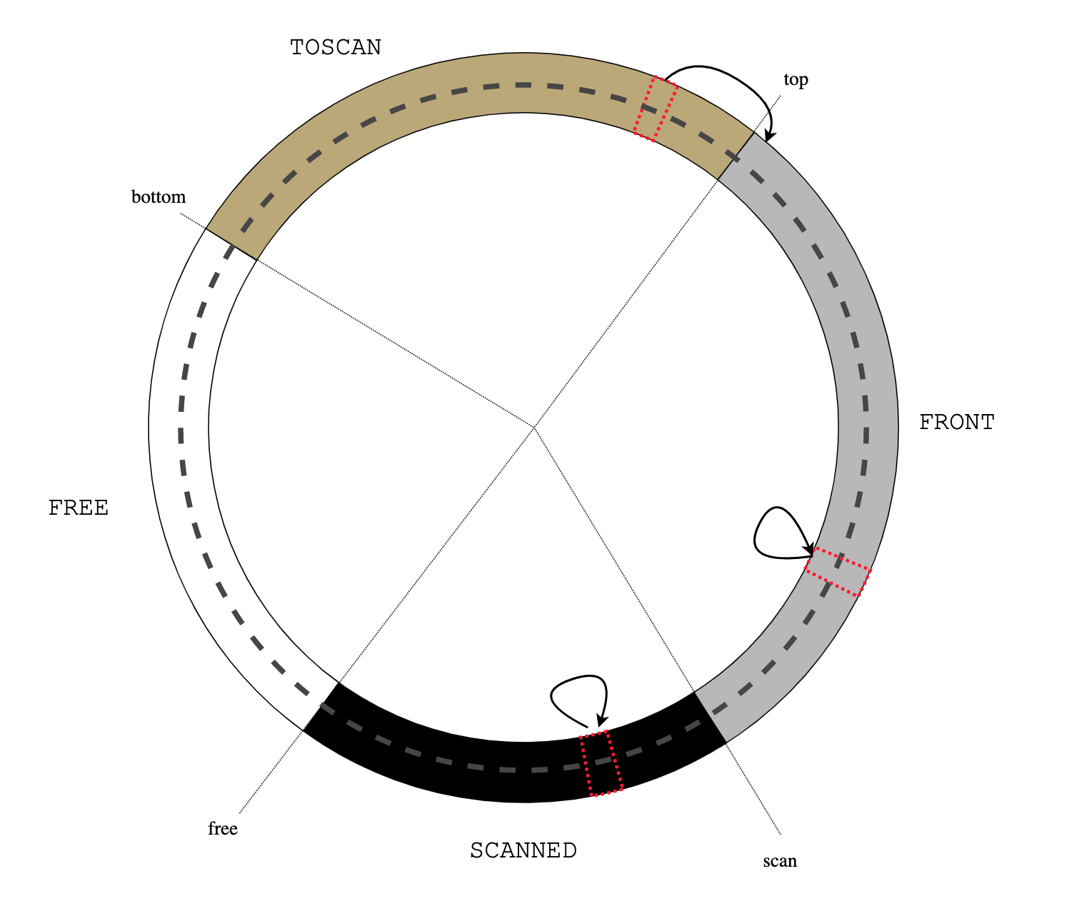
When a black or gray object is read, the read barrier leaves it in place. When an ecru object is read, the barrier un-links the object from the treadmill list (effectively removing it from TOSCAN section) and re-links it to the treadmill either at top or at scan thus making it gray. This barrier guarantees that the mutator cannot violate the invariant simply because the mutator never sees ecru objects (which are grayed by the barrier) and hence cannot store pointers to them anywhere. If the read barrier is present, the write barrier is not necessary.
That's how the invariant is established and maintained by the mutator. We still haven't discussed how the collector works and where these mysterious ecru objects appear from. The collector is very simple: it has a single entry point:
advance() { /* Scan the object pointed to by "scan". */
        for field in pointers(scan) {
                if ecru(scan.field) {
                        darken(scan.field);
                }
        }
        scan := scan.prev; /* Make it black. */
}
advance() takes the gray object pointed to by scan, which is the head of the FRONT list, and grays all ecru objects that this object points to. After that, scan is advanced (counterclockwise), effectively moving the scanned object into the SCANNED section and making it black.
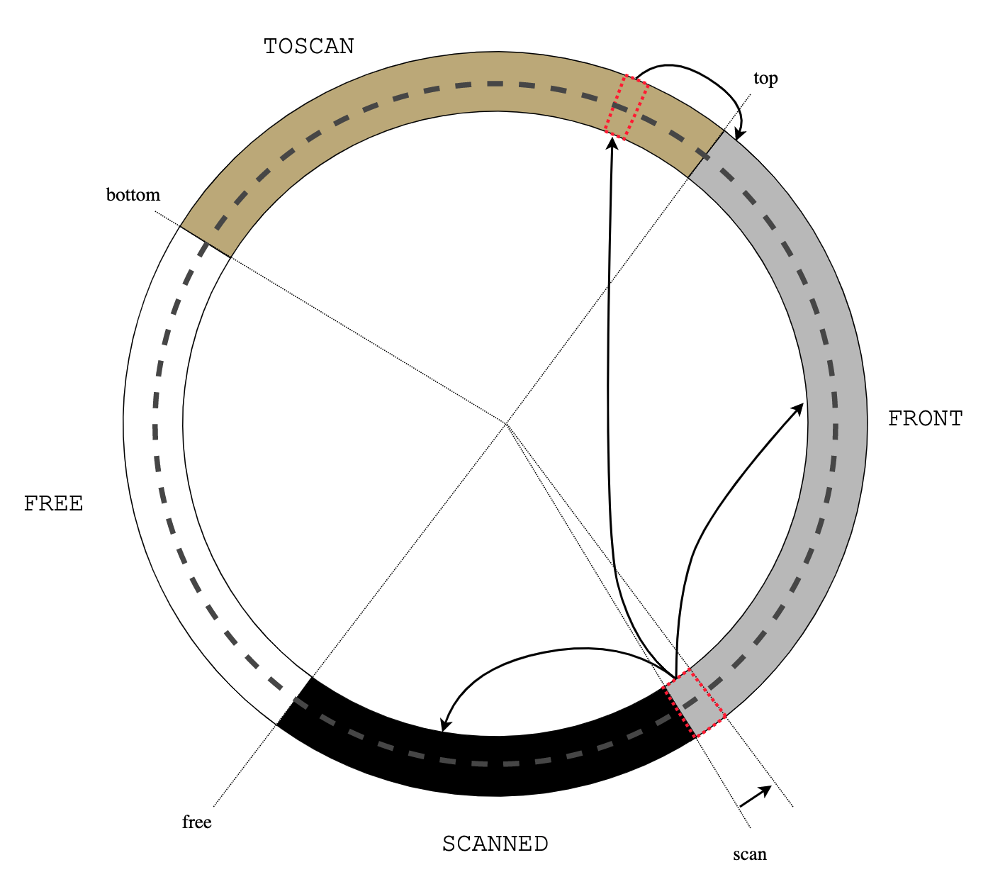
It's not important for now how and when exactly advance() is called. What matters is that it blackens an object while preserving the invariant.
Now comes the crucial part. An allocated object only darkens: the mutator (readbarrier()) and the collector (advance()) can gray an ecru object and advance() blackens a gray object. There is no way for a black object to turn gray or for a gray object to turn ecru. Hence, the total number of allocated non-black objects never increases. But advance() always blackens one object, which means that after some number of calls (interspersed with arbitrary mutator activity), advance() will run out of objects to process: the FRONT section will be empty and there will be no gray objects anymore:
All roots were originally gray and could only darken, so they are now black. And an ecru object is reachable from a black object only through a gray object, but there are no gray objects, so ecru objects are not reachable from roots—they are garbage. This completes the collection cycle and, in principle, it is possible to move all ecru objects to the FREE list at that point and start the next collection cycle. But we can do better. Instead of replenishing the FREE list, wait until all objects are allocated and the FREE list is empty:
Only black and ecru objects remain. Flip them: swap top and bottom pointers and redefine colours: the old black objects are now ecru and the old ecru objects (remember they are garbage) are now white:
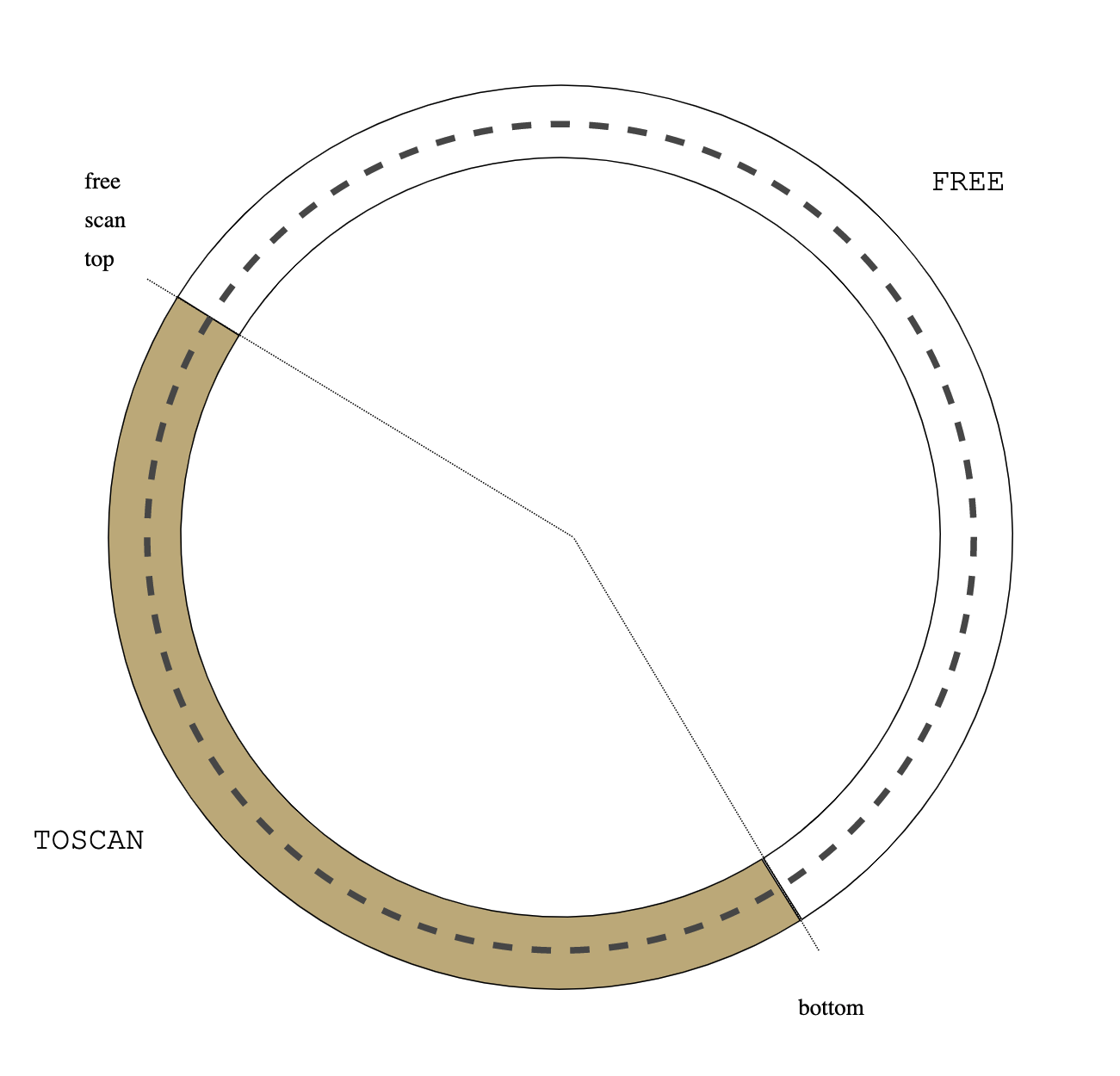
The next collection cycle starts: put the roots between top and scan so that they are the new FRONT:
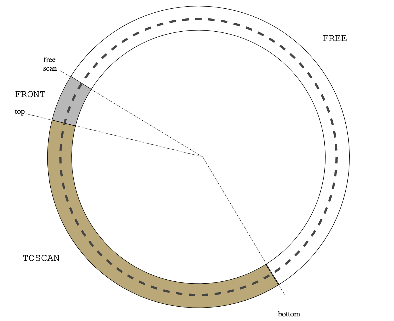
From this point alloc() and advance() can continue as before.
Note that alloc(), advance() and readbarrier() do not actually have to know object colour. They only should be able to tell an ecru (allocated) object from non-ecru, so 1 bit of information per object is required. By waiting until the FREE list is empty and re-defining colours Treadmill avoids the need to scan the objects and change their colours at the end of a collection cycle: it is completely O(1).
The last remaining bit of the puzzle is still lacking: how is it guaranteed that the collection is completed before the FREE list is empty? If the mutator runs out of free objects before the collection cycle is completed, then the only option is to force the cycle to completion by calling advance() repeatedly until there are no more gray objects and then flip, but that's a stop-the-world situation.
The solution is to call advance() from within alloc() guaranteeing scan progress. Baker proved that if advance() is called k times for each alloc() call, then the algorithm never runs out of free objects, provided that the total heap size is at least R*(1 + 1/k) objects, where R is the number of reachable objects.
This completes the Treadmill description.
The algorithm is very flexible. First, the restriction of a single-threaded mutator is not really important: as long as alloc(), advance(), readbarrier() and flip are mutually exclusive, no further constraints on concurrency are necessary. The mutator can be multi-threaded. The collector can be multi-threaded. advance() can be called "synchronously" (from alloc()), explicitly from the mutator code or "asynchronously" from the dedicated collector threads. A feedback-based method can regulate the frequency of calls to advance() depending on the amount of free and garbage objects. alloc() can penalise heavy-allocating threads forcing them to do most of the scanning, etc.
Next, when an object is grayed by darken(), all that matter is that the object is placed in the FRONT section. If darken() places the object next to top, then FRONT acts as a FIFO queue and the scan proceeds in the breadth-first order. If the object is placed next to scan then the scan proceeds in the depth-first order, which might result in a better locality of reference and better performance of a heap in virtual memory. A multi-threaded collector can use multiple FRONT lists, e.g., one per core and scan them concurrently.
New objects can be added to the heap at any time, by atomically linking them somewhere in the FREE list. Similarly, a bunch of objects can be at any moment atomically released from the FREE list with the usual considerations of fragmentation-avoidance in the lower layer allocator.
Support for variable-sized objects requires a separate cyclic list for each size (plus, perhaps an additional overflow list for very large objects). The top, bottom, scan and free pointers become arrays of pointers with an element for each size. If arbitrarily large objects (e.g., arrays) are supported then atomicity of advance() will require additional work: large objects need to be multi-coloured and will blacken gradually.
Forward and backward links to the cyclic list can be embedded in the object header or they can be stored separately, the latter might improve cache utilisation by the scanner.
[0]
Extension.
This post is about set theory, which is a framework to reason about collections, elements and membership.
We start with a informal and naïve outline, which is (very loosely) based on a Godel-Bernays version of set theory. This theory is about sets (collections) which contain elements, which can in turn be sets. When a set \(X\) contains an element \(t\), it is written \(t\in X\).
First, set equality has to be defined:
$$X = Y \equiv (t \in X \equiv t \in Y)$$(Here \(\equiv\) is a logical equivalence, pronounced "if and only if".) This axiom means that sets are equal exactly when they have the same elements. (In this and following formulae, free variables are implicitly universally quantified.)
Subsets are defined by \(X \subseteq Y \equiv (t\in X \Rightarrow t\in Y)\), that is, X is a subset of Y when every element of X is also an element of Y. It's easy to check that \(X = Y \equiv (X\subseteq Y \wedge Y\subseteq X)\), where \(\wedge\) means "and".
Next, a way to build new sets is needed:
E1 Axiom of (extensional) comprehension
$$t \in \{u \mid P(u)\} \equiv P(t)$$This axiom introduces a "set-builder notation" \(\{u \mid P(u) \}\) and states that \(\{u \mid P(u) \}\) is exactly the set of all \(t\) such that \(P(t)\) holds.
Now, there is already enough machinery for two famous collections to be immediately constructed: empty set, \(\varnothing = \{t \mid false \}\), which contains no elements, and the collection of all sets: \(U = \{t \mid true \}\), which contains all possible elements.
With these axioms, conventional set operations can be defined:
singleton: \(\{t\} = \{u\mid u = t\}\), for each \(t\) a singleton set \(\{t\}\) can be constructed that contains \(t\) as its only element. Note that \(t\in\{t\}\)
union: \(X\cup Y = \{t\mid t \in X \vee t \in Y\}\) (\(\vee\) means "or")
intersection: \(X\cap Y = \{t\mid t\in X \wedge t\in Y\}\)
complement: \(\complement X = \{t \mid t \notin X\}\)
(unordered) pair: \(\{t,u\} = \{t\}\cup\{u\}\)
ordered pair: \((t,u) = \{t, \{t, u\}\}\)
power set: \(\mathfrak{P}(X) = \{t \mid t \subseteq X\}\)
From here, one can build hierarchical sets, representing all traditional mathematical structures, starting with natural numbers:
$$0 = \varnothing,\quad 1 = \{0\},\quad 2 = \{0, 1\},\quad \ldots,\quad n + 1 = \{0, \ldots, n\}, \quad \ldots$$then integers, rationals, reals, &c., adding more axioms (of infinity, of foundation, of replacement, &c.) along the way.
It was discovered quite early that this system is not entirely satisfactory. First defect is that it is impossible to have elements which are not sets themselves. For example, one would like to talk about a "set of all inhabited planets in the Solar system". Elements of this set (planets) are not sets, they are called ur-elements. Unfortunately, the axiom of extensionality makes all ur-elements equal to the empty set. Note, that this indicates that the axiom of extensionality doesn't work well with sets that have very few (none) elements. This was never considered a problem, because all sets of interest to mathematics can be constructed without ur-elements.
Another, more serious drawback, arises in the area of very large sets: existence of a set \(\{t\mid t\notin t\}\) directly leads to a contradiction known as Russel's paradox.
Among several possible methods to deal with this, Godel-Bernays version is to separate sets into two types: "smaller" collections which are continued to be called "sets" and "proper classes", which are collections so large that they cannot be a member of any collection. Axiom of comprehension is carefully modified so that set-builder never produces a collection having some class as its element. In this setup Russel's paradox becomes a theorem: \(\{t\mid t\notin t\}\) is a proper class.
Intention.
The axiom of extensionality states that sets are equal when they contain the same elements. What would happen, if set theory were based on a dual notion of intentional equality (which will be denoted by \(\sim\) to tell it from extensional one), where sets are equal when they are contained in the same collections?
I0 Axiom of intensionality:
$$X \sim Y \equiv (X \in t \equiv Y\in t)$$This looks bizarre: for any "normal" set \(X\) a collection of all sets containing \(X\) as element is unmanageably huge. But as a matter of fact, intentional equality is much older than extensional, it is variously known as Leibniz's law, identity of indiscernibles and, in less enlightened age, as duck typing.
There is a nice symmetry: while extensional equality myopically confuses small sets (ur-elements), intensional equality cannot tell very large collections (proper classes) from each other, because they are not members of anything and, therefore, intentionally equal.
The whole extensional theory buildup can be mirrored easily by moving things around \(\in\) sign:
Intensional subsets: \(X \unlhd Y \equiv (X\in t \Rightarrow Y\in t)\)
I1 Axiom of intensional comprehension (incomprehension):
$$[u \mid P(u)]\in t \equiv P(t)$$And associated operations:
uniqum (or should it have been "s-ex-gleton?): \([t] = [u\mid u \sim t]\), note that \([t]\in t\).
intentional union: \(X\triangledown Y = [t\mid X \in t \vee Y \in t]\)
intentional intersection: \(X\triangle Y = [t\mid X \in t \wedge Y \in t]\)
intentional complement: \(\Game X = [t \mid X \notin t]\)
intentional pair: \([t,u] = [t]\triangledown [u]\)
intentional ordered pair: \(<t,u> = [t, [t, u]]\)
intentional power set: \(\mathfrak{J}(X) = [t \mid X \unlhd t\}\)
What do all these things mean? In extensional world, a set is a container, where elements are stored. In intensional world, a set is a property, which other sets might or might not enjoy. If \(t\) has property \(P\), it is written as \(t\in P\). In the traditional notation, \(P\) is called a predicate and \(t\in P\) is written as \(P(t)\). The axiom of intentional equality claims that sets are equal when they have exactly the same properties (quite natural, right?). \(X\) is an intentional subset of \(Y\) when \(Y\) has all properties of \(X\) and perhaps some more (this looks like a nice way to express LSP). Intentional comprehension \([u \mid P(u)]\) is a set having exactly all properties \(t\) for which \(P(t)\) holds and no other properties. Intentional union of two sets is a set having properties of either and their intentional intersection is a set having properties of both, &c. Uniqum \([P]\) is the set that has property \(P\) and no other properties.
Because intensional theory is a perfect dual of extensional nothing interesting is obtained by repeating extensional construction, for example, by building "intensional natural numbers" as
$$0' = U, 1' = [0'], 2' = [0', 1'], \ldots (n + 1)' = [0', \ldots, n'], \ldots$$What is more interesting, is how intensional and extensional twins meet. With some filial affection it seems:
by uniqum property \([\varnothing] \in\varnothing\), which contradicts the definition of \(\varnothing\), also
set \([t\mid false]\) is not a member of any set (perhaps it's a proper class) and set \([t\mid true]\) is a member of every set, which is strange;
a set of which a singleton can be formed has very shallow intentional structure. Indeed:
$$\begin{array}{r@{\;}l@{\quad}} & x \unlhd y \\ \equiv & \text{ \{ definition of intensional subset \} } \\ & x\in t \Rightarrow y\in t \\ \Rightarrow & \text{ \{ substitute \(\{x\}\) for \(t\) \} } \\ & x\in \{x\} \Rightarrow y\in \{x\} \\ \equiv & \text{ \{ \(x\in \{x\}\) is true by the singleton property, modus ponens \} } \\ & y\in \{x\} \\ \equiv & \text{ \{ the singleton property, again \} } \\ & x = y \end{array}$$Like comprehension had to be limited to avoid paradoxes.
To get rid of contradictions and to allow intensional and extensional sets to co-exist peacefully, domains on which singleton and uniqum operations are defined must be narrowed. To be continued.
[Please read the update.]
This repository (https://github.com/nikitadanilov/usched) contains a simple experimental implementation of coroutines alternative to well-known "stackless" and "stackful" methods.
The term "coroutine" gradually grew to mean a mechanism where a computation, which in this context means a chain of nested function calls, can "block" or "yield" so that the top-most caller can proceed and the computation can later be resumed at the blocking point with the chain of intermediate function activation frames preserved.
Prototypical uses of coroutines are lightweight support for potentially blocking operations (user interaction, IO, networking) and generators which produce multiple values (see same fringe problem).
There are two common coroutine implementation methods:
a stackful coroutine runs on a separate stack. When a stackful coroutine blocks, it performs a usual context switch. Historically "coroutines" meant stackful coroutines. Stackful coroutines are basically little more than usual threads, and so they can be kernel (supported by the operating system) or user-space (implemented by a user-space library, also known as green threads), preemptive or cooperative.
a stackless coroutine does not use any stack when blocked. In a typical implementation instead of using a normal function activation frame on the stack, the coroutine uses a special activation frame allocated in the heap so that it can outlive its caller. Using heap-allocated frame to store all local variable lends itself naturally to compiler support, but some people are known to implement stackless coroutines manually via a combination of pre-processing, library and tricks much worse than Duff's device.
Stackful and stateless are by no means the only possibilities. One of the earliest languages to feature generators CLU (distribution) ran generators on the caller's stack.
usched is in some sense intermediate between stackful and stackless: its coroutines do not use stack when blocked, nor do they allocate individual activation frames in the heap.
The following is copied with some abbreviations from usched.c.
Overview
usched: A simple dispatcher for cooperative user-space threads.
A typical implementation of user-space threads allocates a separate stack for each thread when the thread is created and then dispatches threads (as decided by the scheduler) through some context switching mechanism, for example, longjmp().
In usched all threads (represented by struct ustack) are executed on the same "native" stack. When a thread is about to block (usched_block()), a memory buffer for the stack used by this thread is allocated and the stack is copied to the buffer. After that the part of the stack used by the blocking thread is discarded (by longjmp()-ing to the base of the stack) and a new thread is selected. The stack of the selected thread is restored from its buffer and the thread is resumed by longjmp()-ing to the usched_block() that blocked it.
The focus of this implementation is simplicity: the total size of usched.[ch] is less than 120LOC, as measured by SLOCCount.
Advantages:
no need to allocate maximal possible stack at thread initialisation: stack buffer is allocated as needed. It is also possible to free the buffer when the thread is resumed (not currently implemented);
a thread that doesn't block has 0 overhead: it is executed as a native function call (through a function pointer) without any context switching;
because the threads are executed on the stack of the same native underlying thread, native synchronisation primitives (mutices, etc.) work, although the threads share underlying TLS. Of course one cannot use native primitives to synchronise between usched threads running on the same native thread.
Disadvantages:
stack copying introduces overhead (memcpy()) in each context switch;
because stacks are moved around, addresses on a thread stack are only valid while the thread is running. This invalidates certain common programming idioms: other threads and heap cannot store pointers to the stacks, at least to the stacks of the blocked threads. Note that Go language, and probably other run-times, maintains a similar invariant.
Usage
usched is only a dispatcher and not a scheduler: it blocks and resumes threads but
it does not keep track of threads (specifically allocation and freeing of struct ustack instances is done elsewhere),
it implements no scheduling policies.
These things are left to the user, together with stack buffers allocation and freeing. The user supplies 3 call-backs:
usched::s_next(): the scheduling function. This call-backs returns the next thread to execute. This can be either a new (never before executed) thread initialised with ustack_init(), or it can be a blocked thread. The user must keep track of blocked and runnable threads, presumably by providing wrappers to ustack_init() and ustack_block() that would record thread state changes. It is up to usched::s_next() to block and wait for events if there are no runnable threads and all threads are waiting for something;
usched::s_alloc(): allocates new stack buffer of at least the specified size. The user have full control over stack buffer allocation. It is possible to pre-allocate the buffer when the thread is initialised (reducing the cost of usched_block()), it is possible to cache buffers, etc.;
usched::s_free(): frees the previously allocated stack buffer.
rr.h and rr.c provide a simple "round-robin" scheduler implementing all the call-backs. Use it carefully, it was only tested with rmain.c benchmark.
Pictures!
The following diagrams show stack management by usched. The stack grows from right to left.
At the entrance to the dispatcher loop. usched_run(S):
                                                usched_run()
----------------------------------------------+--------------+-------+
                                              | buf | anchor |  ...  |
----------------------------------------------+--------------+-------+
                                              ^
                                              |
                                              sp = S->s_buf
A new (never before executed) thread U is selected by S->s_next(), launch() calls the thread startup function U->u_f():
                               U->u_f() launch() usched_run()
 -----------------------------+---------+-----+--------------+-------+
                              |         | pad | buf | anchor |  ...  |
 -----------------------------+---------+-----+--------------+-------+
                              ^         ^
                              |         |
                              sp        U->u_bottom
The thread executes as usual on the stack, until it blocks by calling usched_block():
    usched_block()       bar() U->u_f() launch() usched_run()
 ----------+------+-----+-----+---------+-----+--------------+-------+
           | here | ... |     |         | pad | buf | anchor |  ...  |
 ----------+------+-----+-----+---------+-----+--------------+-------+
      ^    ^                            ^
      |    +-- sp = U->u_cont           |
      |                                 U->u_bottom
      U->u_top
The stack from U->u_top to U->u_bottom is copied into the stack buffer U->u_stack, and control returns to usched_run() by longjmp(S->s_buf):
                                                usched_run()
----------------------------------------------+--------------+-------+
                                              | buf | anchor |  ...  |
----------------------------------------------+--------------+-------+
                                              ^
                                              |
                                              sp = S->s_buf
Next, suppose S->s_next() selects a previously blocked thread V ready to be resumed. usched_run() calls cont(V).
                                        cont()  usched_run()
----------------------------------------+-----+--------------+-------+
                                        |     | buf | anchor |  ...  |
----------------------------------------+-----+--------------+-------+
                                        ^
                                        |
                                        sp
cont() copies the stack from the buffer to [V->u_top, V->u_bottom] range. It's important that this memcpy() operation does not overwrite cont()'s own stack frame, this is why pad[] array is needed in launch(): it advances V->u_bottom and gives cont() some space to operate.
  usched_block()       foo() V->u_f()   cont()  usched_run()
---------+------+-----+-----+--------+--+-----+--------------+-------+
         | here | ... |     |        |  |     | buf | anchor |  ...  |
---------+------+-----+-----+--------+--+-----+--------------+-------+
    ^    ^                           ^  ^
    |    +-- V->u_cont               |  +-- sp
    |                                |
    V->u_top                         V->u_bottom
Then cont() longjmp()-s to V->u_cont, restoring V execution context:
  usched_block()       foo() V->u_f()   cont()  usched_run()
---------+------+-----+-----+--------+--+-----+--------------+-------+
         | here | ... |     |        |  |     | buf | anchor |  ...  |
---------+------+-----+-----+--------+--+-----+--------------+-------+
         ^
         +-- sp = V->u_cont
V continues its execution as if it returned from usched_block().
Multiprocessing
By design, a single instance of struct usched cannot take advantage of multiple processors, because all its threads are executing within a single native thread. Multiple instances of struct usched can co-exist within a single process address space, but a ustack thread created for one instance cannot be migrated to another. One possible strategy to add support for multiple processors is to create multiple instances of struct usched and schedule them (that is, schedule the threads running respective usched_run()-s) to processors via pthread_setaffinity_np() or similar. See rr.c for a simplistic implementation.
Current limitations
the stack is assumed to grow toward lower addresses. This is easy to fix, if necessary;
the implementation is not signal-safe. Fixing this can be as easy as replacing {set,long}jmp() calls with their sig{set,long}jmp() counterparts. At the moment signal-based code, like gperf -lprofiler library, would most likely crash usched;
usched.c must be compiled without optimisations and with -fno-stack-protector option (gcc);
usched threads are cooperative: a thread will continue to run until it completes of blocks. Adding preemption (via signal-based timers) is relatively easy, the actual preemption decision will be relegated to the external "scheduler" via a new usched::s_preempt() call-back invoked from a signal handler.
Notes
Midori seems to use a similar method: a coroutine (called activity there) starts on the native stack. If it needs to block, frames are allocated in the heap (this requires compiler support) and filled in from the stack, the coroutine runs in these heap-allocated frames when resumed.
Benchmarks
usched was benchmarked against a few stackful (go, pthreads) and stackless (rust, c++ coroutines) implementations. A couple of caveats:
all benchmarking in general is subject to the reservations voiced by Hippocrates and usually translated (with the complete reversal of the meaning) as ars longa, vita brevis, which means: "the art [of doctor or tester] takes long time to learn, but the life of a student is brief, symptoms are vague, chances of success are doubtful";
the author is much less than fluent with all the languages and frameworks used in the benchmarking. It is possible that some of the benchmarking code is inefficient or just outright wrong. Any comments are appreciated.
The benchmark tries to measure the efficiency of coroutine switching. It creates R cycles, N coroutines each. Each cycle performs M rounds, where each round consists of sending a message across the cycle: a particular coroutine (selected depending on the round number) sends the message to its right neighbour, all other coroutines relay the message received from the left to the right, the round completes when the originator receives the message after it passed through the entire cycle.
If N == 2, the benchmark is R pairs of processes, ping-ponging M messages within each pair.
Some benchmarks support two additional parameters: D (additional space in bytes, artificially consumed by each coroutine in its frame) and P (the number of native threads used to schedule the coroutines.
The benchmark creates N*R coroutines and sends a total of N*R*M messages, the latter being proportional to the number of coroutine switches.
bench.sh runs all implementations with the same N, R and M parameters. graph.py plots the results.
POSIX. Source: pmain.c, binary: pmain. Pthreads-based stackful implementation in C. Uses default thread attributes. pmain.c also contains emulation of unnamed POSIX semaphores for Darwin. Plot label: "P". This benchmarks crashes with "pmain: pthread_create: Resource temporarily unavailable" for large values of N*R.
Go. Source: gmain.go, binary: gmain. The code is straightforward (it was a pleasure to write). P is supported via runtime.GOMAXPROCS(). "GO1T" are the results for a single native thread, "GO" are the results without the restriction on the number of threads.
Rust. Source: cycle/src/main.rs, binary: cycle/target/release/cycle. Stackless implementation using Rust builtin async/.await. Label: "R". It is single-threaded (I haven't figured out how to distribute coroutines to multiple executors), so should be compared with GO1T, C++1T and U1T. Instead of fighting with the Rust borrow checker, I used "unsafe" and shared data-structures between multiple coroutines much like other benchmarks do.
C++. Source: c++main.cpp, binary: c++main. The current state of coroutine support in C++ is unclear. Is everybody supposed to directly use <coroutine> interfaces or one of the mutually incompatible libraries that provide easier to use interfaces on top of <coroutine>? This benchmark uses Lewis Baker's cppcoro, (Andreas Buhr's fork). Labels: "C++" and "C++1T" (for single-threaded results).
usched. Source: rmain.c, binary: rmain. Based on usched.[ch] and rr.[ch] This is our main interest, so we test a few combinations of parameters.
Label: "U": the default configuration, round-robin scheduler over 16 native threads,
"U1K": 1000 bytes of additional stack space for each coroutine
"U10K": 10000 bytes,
"U1T": round-robin over 1 native thread,
"U1TS": round-robin over 1 native thread with pthread locking in rr.c compiled out (-DSINGLE_THREAD compilation option, a separate binary rmain.1t).
Update "UL": uses "local" scheduler ll.c. All coroutines within a cycle are assigned to the same native thread so that scheduling between them require no locking. This demonstrates very high throughput (comparable to C++), but unfortunately I do not have time right now to re-do all the measurements consistently. Binary: lmain.
bench.sh runs all benchmarks with N == 2 (message ping-pong) and N == 8. Raw results are in results.linux. In the graphs, the horizontal axis is the number of coroutines (N*R, logarithmic) and the vertical axis is the operations (N*R*M) per second.
Environment: Linux VM, 16 processors, 16GB of memory. Kernel: 4.18.0 (Rocky Linux).
(N == 8) A few notes:
As mentioned above, pthreads-based solution crashes with around 50K threads.
Most single-threaded versions ("GO1T", "R" and "U1T") are stable as corpse's body temperature. Rust cools off completely at about 500K coroutines. Single-threaded C++ ("C++1T") on the other hand is the most performant solution for almost the entire range of measurement, it is only for coroutine counts higher than 500K when "U" overtakes it.
It is interesting that a very simple and unoptimised usched fares so well against heavily optimized C++ and Go run-times. (Again, see the reservations about the benchmarking.)
Rust is disappointing: one would hope to get better results from a rich type system combined with compiler support.
(N == 2)
First, note that the scale is different on the vertical axis.
Single-threaded benchmarks display roughly the same behaviour (exactly the same in "C++1T" case) as with N == 8.
Go is somewhat better. Perhaps its scheduler is optimised for message ping-pong usual in channel-based concurrency models?
usched variants are much worse (50% worse for "U") than N == 8.
Rust is disappointing.
To reproduce:
$ # install libraries and everything, then...
$ make
$ while : ;do ./bench.sh | tee -a results; sleep 5 ;done # collect enough results, this might take long...
^C
$ grep -h '^ *[2N],' results | python3 graph.py c2.svg > c2-table.md # create plot for N == 2
$ grep -h '^ *[8N],' results | python3 graph.py c8.svg > c8-table.md # create plot for N == 8
Conclusion
Overall, the results are surprisingly good. The difference between "U1T" and "U1TS" indicates that the locking in rr.c affects performance significantly, and affects it even more with multiple native threads, when locks are contended across processors. I'll try to produce a more efficient (perhaps lockless) version of a scheduler as the next step.
usched is a light-weight cooperative-multitasking-coroutine library that I wrote (github.com). To switch between threads, it copies the stack of the outgoing thread out to somewhere (e.g., the heap) and copies in the stack of the incoming thread, that was similarly copied out on the previous context switch.
As usual, whatever you invent, eventually turns out to be known since long time ago. In this case, we are talking about something that happened at fabulous times, almost at the dawn of history, as far as computing technology is concerned: Algol-68. Dr. J.J.F.M. Schlichting's PhD. thesis Een Vroege Implementatie Van Herzien Algol 68 (An Early Implementation Of Revised Algol 68) describes in detail an implementation of that language by Control Data B. Y. and the University of Amsterdam (among others).
On p. 4-30 we find:
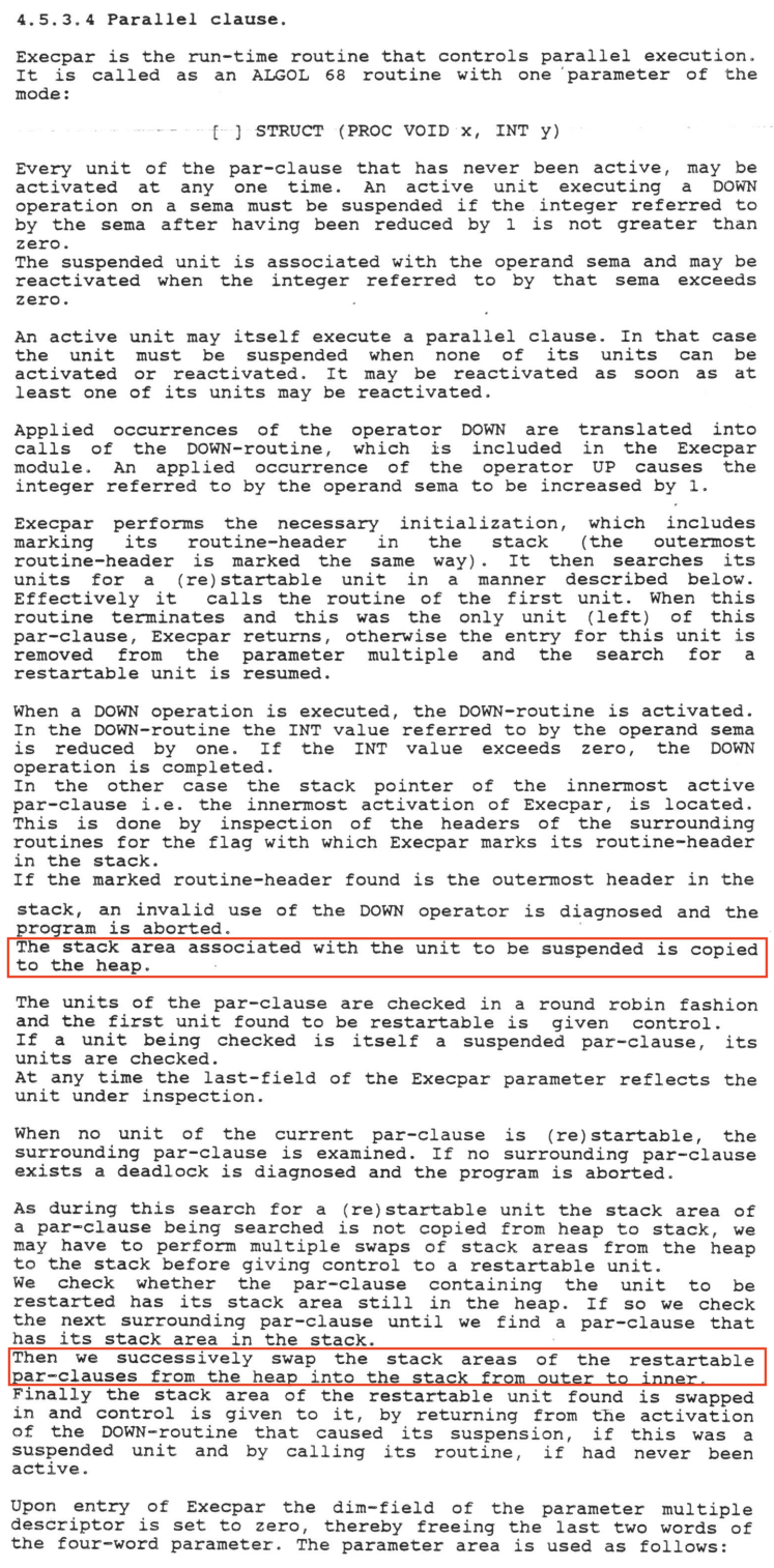
The term thread is not used (maybe not yet invented, definitely not current), but we see a sophisticated compiler-assisted cooperative multitasking with fork-join concurrency and cactus stacks:
[0]
Update for the previous post about stackswap coroutine implementation usched.
To recap, usched is an experimental (and very simple, 120LOC) coroutine implementation different from stackful and stackless models: coroutines are executed on the native stack of the caller and when the coroutine is about to block its stack is copied into a separately allocated (e.g., in the heap) buffer. The buffer is copied back onto the native stack when the coroutine is ready to resume.
I added a new scheduler ll.c that distributes coroutines across multiple native threads and then does lockless scheduling within each thread. In the benchmark (the same as in the previous post), each coroutine in the communicating cycle belongs to the same thread.
Results are amazing: usched actually beats compiler-assisted C++ coroutines by a large margin. The horizontal axis is the number of coroutines in the test (logarithmic) and the vertical axis is coroutine wakeup-wait operations per second (1 == 1e8 op/sec).
I only kept the most efficient implementation from every competing class: C++ for stackless, GO for stackful and usched for stackswap. See the full results in results.darwin
Consider a system describing possible computations (e.g., a programming language or a state machine formalism) including interactions with the external world, that is, input and output facilities.
A pair of dual sub-classes of computational elements (values, objects, functions, &c.) can be defined:
finitary elements that are known to not depend on input and
ideal elements that output is known to not depend on.
The rest of elements may depend on input and may affect output. Let's call such elements laic ("temporal" might be a better word).
The class of finitary elements is well-known: because they can be computed without input, they can be computed before the program starts, i.e., they correspond to various constants, including static entities like types (in statically typed languages), classes, function bodies and so on. Some languages have powerful finitary computations, for example, C++ template specialisation is Turing complete.
Laic elements are the most usual things like variables and objects.
Ideal elements are less known. They have a long history of use in the area of formal program verification where they are called ghost or auxiliary variables.
There is an obvious restriction of data and control flow between various types of elements:
finitary element may depend only on finitary elements;
laic element may depend on laic and finitary elements (e.g., normal function can take a constant as a parameter, but constant cannot be initialised with the value of a variable or function call);
ideal element may depend on any element (e.g., ideal variable can be assigned the value of a laic variable, but not other way around).
The most important property of ideal elements is that, because they don't affect observable program behaviour, there is no need to actually compute them! Yet, they are useful exactly because of this property: ideal elements are not computed and, hence, are not constrained by the limitations of actual computational environments. For example, an ideal variable can represent an infinite (even uncountable) collection or a real number (real real number, not approximation); an ideal function can be defined by the transfinite induction or by a formula involving quantifiers.
To use ideal elements, one assumes that they follow normal rules of the language (for example, axiomatic or denotational semantics). This assumption doesn't burden the implementors of the language precisely because the ideal elements are not computed. Under that assumption, one can reason about properties of ideal elements.
As a simplest example, an ideal variable can be used to record the sequence of calls to a certain function:
ideal f_seq = {};
function f(arg) {
        f_seq := f_seq ++ arg;
        ...
};
and then reason about f_seq using whatever method is used to reason about laic elements (e.g., weakest preconditions, Hoare triples or usual hand-waving), for example, to prove that messages delivered to a receiver were sent by the sender (that is, deliver_seq is a sub-sequence of send_seq).
It is interesting that both finitary elements (specifically, static types) and ideal elements help to reason about the behaviour of the laic world sandwiched between them.
Nothing in this short article is new, except for the (obvious) duality between ideal and finitary elements.
Exercise 0: implement linear types by casting laic elements to ideal.
Exercise 1: implement garbage collection similarly.
Dedicated to VM and file system developers and researches...
It is immediately apparent from these figures that moving-arm disks should never be used, neither for paging applications nor for any other heavy-traffic auxiliary memory applications.
Peter J. Denning -- Virtual Memory.
I added a bit of material to the Wikipedia entry on Page replacement algorithms: a bit of history, precleaning, global vs. local replacement, description of LRU degradation for cyclic access patterns, random replacement, links to the modern algorithms, unification of VM with file system cache, etc. Original entry was more or less re-hash of a section from Tannenbaum's "Operating Systems".
Subject: [ntdev] WdfUsbTargetDeviceSendControlTransferSynchronously and timeouts
update: Like this wasn't enough.
Below are excerpts from
find . -name \*dll |\
        xargs strings -- |\
        grep -i '^[a-z0-9_]*$' |\
        awk '{ print length($1) "\t" $1 }' |\
        sort -n
output (executed in WinXP system directory):
50      ZwAccessCheckByTypeResultListAndAuditAlarmByHandle
51      Java_NPDS_npDSJavaPeer_SetSendMouseClickEvents_stub
51      Java_NPDS_npDSJavaPeer_SetShowPositionControls_stub
51      JET_errDistributedTransactionNotYetPreparedToCommit
52      ACTIVATION_CONTEXT_SECTION_COM_INTERFACE_REDIRECTION
52      ConvertSecurityDescriptorToStringSecurityDescriptorA
52      ConvertSecurityDescriptorToStringSecurityDescriptorW
53      ACTIVATION_CONTEXT_SECTION_GLOBAL_OBJECT_RENAME_TABLE
55      ACTIVATION_CONTEXT_SECTION_COM_TYPE_LIBRARY_REDIRECTION
55      SxspComProgIdRedirectionStringSectionGenerationCallback
56      Java_NPDS_npDSJavaPeer_GetSendOpenStateChangeEvents_stub
56      Java_NPDS_npDSJavaPeer_GetSendPlayStateChangeEvents_stub
56      SxspComTypeLibRedirectionStringSectionGenerationCallback
57      SxspComputeInternalAssemblyIdentityAttributeBytesRequired
57      SxspWindowClassRedirectionStringSectionGenerationCallback
62      SxspComputeInternalAssemblyIdentityAttributeEncodedTextualSize
62      SxspGenerateTextuallyEncodedPolicyIdentityFromAssemblyIdentity
64      RtlpQueryAssemblyInformationActivationContextDetailedInformation
71      RtlpQueryFilesInAssemblyInformationActivationContextDetailedInformation
which probably gives us the champion.
As a comparison, for linux-2.6.15
find . -type f -follow -name '*.[chS]' |\
        xargs grep -hi '[a-z0-9_]\{70,\}' -- /dev/null
gives:
70 ZORRO_PROD_PHASE5_BLIZZARD_1230_II_FASTLANE_Z3_CYBERSCSI_CYBERSTORM060So windows is one character closer to hell than linux.
[2025/05/17] Update: _OpenLogicalChannelAck_reverseLogicalChannelParameters_multiplexParameters, no comment.
[Updated: 2005.07.24]
The key point of working set algorithm is not virtual time relative to which recently used pages are defined. Virtual time is a problem rather than a solution. At the time when working set algorithm was designed, there was one to one mapping between address spaces and threads. In such setup virtual time based scanning ties memory scheduling and processor scheduling and, hence, avoids thrashing, which is a situation when one resource (processor) is scheduled to achieve its maximal utilization, ignoring constraints imposed by other resource (memory) (See Dijkstra papers EWD408 and EWD462 for as always lucid an explanation).
In modern systems there is no such one to one mapping anymore. There are multiple threads executing within the same address space. There are memory consumers that are not readily identifiable with any execution context at all: file system cache (which is merged with VM in any self-respecting kernel), general in-kernel memory allocator, etc. It means that:
there is no relevant notion of virtual time to be used during scanning;
working set control fails to bind memory and processor scheduling together, which will decrease its effectiveness.
One extreme case is to consider whole system as one entity. Then virtual time degenerates into physical one, and working set algorithm into active/inactive queue.
Moreover, working set is not page replacement algorithms at all. That is, it doesn't answer to the question "System is low on memory, what page should be reclaimed?"; Instead it vaguely points to some address space and proposes to reclaim some unknown page from it. This made sense for the time-shared server running large number of tasks with disjoint address spaces, but for the modern system working set algorithm will be most likely finger-pointing to the Mozilla (or OpenOffice, or...) on the client and Apache (or Oracle, or...) on the server. Which is completely useless, because we still don't know what page is to be reclaimed.
XNU (OSX kernel) VM scanner marks vnodes as (vp->v_flag & VHASBEENPAGED). write(2) path checks for this and sends all dirty pages for this vnode down the pipe if this flags is set. Reason:
/*
 * this vnode had pages cleaned to it by
 * the pager which indicates that either
 * it's not very 'hot', or the system is
 * being overwhelmed by a lot of dirty
 * data being delayed in the VM cache...
 * in either event, we'll push our remaining
 * delayed data at this point...  this will
 * be more efficient than paging out 1 page at
 * a time, and will also act as a throttle
 * by delaying this client from writing any
 * more data until all his delayed data has
 * at least been queued to the uderlying driver.
 */

(студенческая олимпиада МФТИ по математике, 2013, задача 3)
Предположим, что \(\forall x\in\mathbb{R}\to f(x) \neq 0\). Возьмем произвольный интервал \([a, b] \subset \mathbb{R}\), \(a \lt b\) и докажем, что на этом интервале есть точка \(x_0\) такая, что \(\lim \limits_{x\to x_0} f(x) \neq 0\).
Пусть \(T_n = |f|^{-1}([\frac{1}{n}, +\infty)) \cap [a, b]\), т.е. \(x \in T_n \equiv |f(x)| \ge \frac{1}{n} \wedge x\in[a, b]\), для \(n > 0\).
Если каждое \(T_n\) нигде неплотно, нигде неплотно и их объединение, (т.к. \([a, b]\) — бэровское пространство), но их объединение это весь интервал \([a, b]\) — противоречие. Следовательно, некоторое \(T_n\) имеет внутреннюю точку, \(x_0 \in T_n\), тогда \(T_n\) содержит \(x_0\) вместе с неким открытым интервалом на котором, таким образом, \(|f(x)| ≥ \frac{1}{n}\), и, следовательно, \(|\lim \limits_{x\to x_0} f(x)| \ge \frac{1}{n} \gt 0\).
Заметим, что мы доказали больше, чем требовалось, а именно, что множество нулей всюду плотно. Или, что функция всюду сходящаяся к непрерывной, почти всюду непрерывна (замените \(0\) на произвольную непрерывную \(g:\mathbb{R}\to\mathbb{R}\)).
(2014.12.15) Обобщение.
Let \(X\) be a Baire space, \(Y\)—a second-countable Urysohn space and \(f,g : X \to Y\)—arbitrary maps. If \((\forall x\in X)(\lim\limits_{t\to x}f(t) = \lim\limits_{t\to x}g(t))\) then \(f = g\) on a dense subset.
Proof (by contraposition). Suppose that there is an open \(A \subseteq X\), such that \((\forall x\in A)(f(x)\neq g(x))\). Let \(B\) be a countable base of \(Y\).
Define a countable family of subsets of \(A\): \(T_{U,V} = f^{-1}(U) \cap g^{-1}(V) \cap A\), where \(U, V \in B\) (that is, \(U\) and \(V\) are open subsets of \(Y\)). For any \(x\in A\), \(f(x)\neq g(x)\), and because \(Y\) is Urysohn, there are \(U, V\in B, cl(U)\cap cl(V) = \varnothing, f(x)\in U, g(x)\in V\), that is, \(x\in T_{U,V}\) that is,
$$\bigcup\limits_{cl(U)\cap cl(V) = \varnothing} T_{U,V} = A$$Because \(X\) and hence \(A\) are Baire spaces, one of \(T_{U,V}\) in the union above, say \(T_{U_0, V_0}\) is not nowhere dense. That is, there is an open set \(G\subseteq A\) such that for any \(x_0\in G\), and any open neighbourhood \(S, x_0\in S\), \(S \cap T_{U_0,V_0}\neq\varnothing\), that is there exists a \(x'\in S\) such that \(f(x') \in U_0\) and \(g(x')\in V_0\).
Suppose that \(\lim\limits_{t\to x_0}f(t) = \lim\limits_{t\to x_0}g(t) = y\in Y\). This means that every open neighbourhood of \(y\) intersects with \(U_0\), hence \(y\in cl(U_0)\). Similarly \(y\in cl(V_0)\), contradiction with \(cl(U_0)\cap cl(V_0) = \varnothing\). End of proof.
PS: для задачи 2, ответ \(k = 2\cdot n - 2\).
"Усердие все превозмогает!"
К. Прутков, Мысли и афоризмы, I, 84
In C and C++ a static variable can be defined in a function scope:
int foo() {
        static int counter = 1;
        printf("foo() has been called %i times.\n", counter++);
        ...
}
Technically, this defines counter as an object of static storage duration that is allocated not within the function activation frame (which is typically on the stack, but can be on the heap for a coroutine), but as a global object. This is often used to shift computational cost out of the hot path, by precomputing some state and storing it in a static object.
When exactly a static object is initialised?
For C this question is vacuous, because the initialiser must be a compile-time constant, so the actual value of the static object is embedded in the compiled binary and is always valid.
C++ has a bizarrely complicated taxonomy of initialisations. There is static initialisation, which roughly corresponds to C initialisation, subdivided into constant-initialisation and zero-initialisation. Then there is dynamic initialisation, further divided into unordered, partially-ordered and ordered categories. None of these, however, captures our case: for block-local variables, the Standard has a special sub-section in "Declaration statement" [stmt.dcl.4]:
Dynamic initialization of a block-scope variable with static storage duration or thread storage duration is performed the first time control passes through its declaration; such a variable is considered initialized upon the completion of its initialization. If the initialization exits by throwing an exception, the initialization is not complete, so it will be tried again the next time control enters the declaration. If control enters the declaration concurrently while the variable is being initialized, the concurrent execution shall wait for completion of the initialization. If control re-enters the declaration recursively while the variable is being initialized, the behavior is undefined.
For example in
struct Bar {
        Bar() : var(1) {}
        int var;
};

int foo(int x) {
        static Bar b{};
        return b.var + 1;
}
the constructor for b should be called exactly once when foo() is called the first time. This initialisation semantics is very close (sans the exceptions part) to pthread_once(). It is clear that the compiler must add some sort of an internal flag to check whether the initialisation has already been performed and some synchronisation object to serialise concurrent calls to foo() [godbolt]:
foo(int):
        push    rbp
        mov     rbp, rsp
        sub     rsp, 16
        mov     DWORD PTR [rbp-4], edi
        movzx   eax, BYTE PTR guard variable for foo(int)::b[rip]
        test    al, al
        sete    al
        test    al, al
        je      .L3
        mov     edi, OFFSET FLAT:guard variable for foo(int)::b
        call    __cxa_guard_acquire
        test    eax, eax
        setne   al
        test    al, al
        je      .L3
        mov     edi, OFFSET FLAT:foo(int)::b
        call    Bar::Bar() [complete object constructor]
        mov     edi, OFFSET FLAT:guard variable for foo(int)::b
        call    __cxa_guard_release
.L3:
        mov     eax, DWORD PTR foo(int)::b[rip]
        add     eax, 1
        leave
        ret
This corresponds roughly to the following code:
int foo(int x) {
        static Bar b{};
        static std::atomic<int> __b_guard = 1;
        if (__b_guard != 0 && __cxa_guard_acquire(&__b_guard) != 0) {
                new (&b) Bar{}; /* Construct b in-place. */
                __cxa_guard_release(&__b_guard)
        }
        return b.var + 1;
}
Here __b_guard (guard variable for foo(int)::b in assembly) is the flag variable added by the compiler. __cxa_guard_acquire() is a suprisingly complex function, which includes its own synchronisation mechanism implemented directly on top of the raw Linux futex syscall.
On the first call to foo() initialisation incurs a function call to __cxa_guard_acquire(), plus atomic_load_explicit(&__b_guard, memory_order::acquire) in __cxa_guard_acquire(). On ARM, such atomic load incurs a memory barrier---a fairly expensive operation.
Even after the static variable has been initialised, an additional conditional branch (je .L3) is required every time.
Can this additional cost be reduced? Yes, in fact it can be completely eliminated, making block-level static variables exactly as efficient as file-level ones. For this we need a certain old, but little-known feature of UNIX linkers. From GNU binutils documentation (beware than in the old versions the terminating symbol is mistakenly referred to as __end_SECNAME):
If an output section’s name is the same as the input section’s name and is representable as a C identifier, then the linker will automatically PROVIDE two symbols: __start_SECNAME and __stop_SECNAME, where SECNAME is the name of the section. These indicate the start address and end address of the output section respectively. Note: most section names are not representable as C identifiers because they contain a ‘.’ character.
(Solaris linker calls them "Encapsulation Symbols", see here.)
The idea is the following: instead of defining a block-level static instance of Bar, define a trivially-initialisable object of a size sufficient to hold an instance of Bar in a dedicated section STATIC_Bar, via (more or less portable) __attribute__((section)). Only such place-holder objects and nothing else are placed in this section. Then, during global static initialisation, scan the resulting array of place-holder objects from __start_STATIC_Bar to __stop_STATIC_Bar and initialise Bar instances in-place. Assuming that functions where static Bars are defined are not themselves called during global static initialisation, this would initialise everything correctly: by the time foo() is called, its b has already been initialised.
Something like this:
#include <stdio.h>
#include <new> /* For placement new. */

#define FAST_STATIC(T)                                                                    \
*({                                                                                       \
        struct placeholder {                                                              \
            alignas(T) char buf[sizeof(T)];                                               \
        };                                                                                \
        static constinit placeholder ph __attribute__((section ("STATIC_" #T))) {{}};     \
        reinterpret_cast<T *>(ph.buf);                                                    \
})

template <typename T> static int section_init(T *start, T *stop)
{
        for (T *s = start; s < stop; ++s)
            new (s) T; /* Construct in-place. */
        return 0;
}

#define FAST_STATIC_INIT(T)                                     \
extern "C" T __start_STATIC_ ## T;                              \
extern "C" T __stop_STATIC_ ## T;                               \
static int _init_ ## T = section_init<T>(&__start_STATIC_ ## T, \
                                         &__stop_STATIC_ ## T);

struct Bar {
        Bar() : var(1) {}
        int var;
};

int foo(int x) {
        Bar &b0 = FAST_STATIC(Bar);
        Bar &b1 = FAST_STATIC(Bar);
        return b0.var + b1.var + 1;
}

FAST_STATIC_INIT(Bar);

int main(int argc, char **argv) {
        return printf("%i\n", foo(argc)); /* Prints "3". */
}
Check the resulting assembly [godbolt]:
foo(int)::ph:
        .zero   4
foo(int)::ph:
        .zero   4
foo(int):
        push    rbp
        mov     rbp, rsp
        mov     DWORD PTR [rbp-20], edi
        mov     QWORD PTR [rbp-8], OFFSET FLAT:foo(int)::ph
        mov     QWORD PTR [rbp-16], OFFSET FLAT:foo(int)::ph
        mov     rax, QWORD PTR [rbp-8]
        mov     edx, DWORD PTR [rax]
        mov     rax, QWORD PTR [rbp-16]
        mov     eax, DWORD PTR [rax]
        add     eax, edx
        add     eax, 1
        pop     rbp
retVoilà! The "is-initialised" branch and the calls to __cxa_guard_acquire() are gone, yet b0 and b1 are initialised before foo() is called, just as we want. But not so fast, it's C++.
Let's add another static Bar instance, this time in an inline function:
int inline baz(int x) {
        Bar &b = FAST_STATIC(Bar);
        return b.var * x;
}
GCC reports [godbolt]:
<source>:9:38: error: 'ph' causes a section type conflict with 'ph' in section 'STATIC_Bar'(clang works fine [godbolt], by the way.)
The problem is that in addition to name, sections output by the compiler also have attributes. The compiler selects the attributes based on the properties of the scope where the symbol (to which __attribute__((section)) is applied) is defined. Inline functions force a different attribute selection (similarly do template members), and the linker ends up with multiple sections with the same name, but conflicting attributes. See stackoverflow for details.
As it is, FAST_STATIC() is usable, but section attribute conflicts put awkward resrictions on its applicability. Is this the best we can do? For some time I thought that it is, but then I realised that there is another way to specify the section in which the variable is located: the .pushsection directive of the embedded assembler (do not be afraid, we will use only portable part).
If you do something like
__asm__(".pushsection STATIC_Bar,\"aw\",@progbits\n" \
        ".quad " symbol "\n"                         \
        ".popsection\n")
then the address of the symbol is placed in STATIC_Bar section with the specified attributes.
All we need is something like
#define FAST_STATIC(T)                                          \
*({                                                             \
        struct placeholder {                                    \
            alignas(T) char buf[sizeof(T)];                     \
        };                                                      \
        static constinit placeholder ph {{}};                   \
        __asm__(".pushsection STATIC_" #T ",\"aw\",@progbits\n" \
                ".quad ph\n"                                    \
                ".popsection\n");                               \
        reinterpret_cast<T *>(ph.buf);                          \
})
and we are good (section_init() needs to be fixed a bit, because STATIC_Bar now contains pointers, not instances). But not so fast, it's C++. This does not even compile [godbolt]:
ld: /tmp/ccZRzXXj.o:(STATIC_Bar+0x0): undefined reference to `ph'
ld: /tmp/ccZRzXXj.o:(STATIC_Bar+0x8): undefined reference to `ph'
ld: /tmp/ccZRzXXj.o:(STATIC_Bar+0x10): undefined reference to `ph'
collect2: error: ld returned 1 exit status
Execution build compiler returned: 1
When you define static constinit placeholder ph, the actual name the compiler uses for the symbol is not ph it is the mangled version of something like foo(int)::ph that we saw in the assembly listing above. There is no ph for .quad ph to resolve to.
OK. Are we stuck now? In fact not. You can instruct the compiler to use a particular symbol name, instead of the mangled one. With
int foo asm ("bar") = 2;the compiler will use "bar" as the symbol name for foo (both gcc and clang support this).
Of course if we just do
static constinit placeholder ph asm("ph") {{}};we fall in the opposite trap of having multiple definitions for "ph". We need to define unique names for our symbols, but there is more or less standard trick for this, based on __COUNTER__ macro. We also need a couple of, again standard, macros for concatenation and stringification. The final version looks like this:
#define CAT0(a, b) a ## b
#define CAT(a, b) CAT0(a, b)

#define STR0(x) # x
#define STR(x) STR0(x)

#define FAST_STATIC_DO(T, id)                                   \
*({                                                             \
        struct placeholder {                                    \
            alignas(T) char buf[sizeof(T)];                     \
        };                                                      \
        static constinit placeholder id asm(STR(id)) {{}};      \
        __asm__(".pushsection STATIC_" #T ",\"aw\",@progbits\n" \
                ".quad " STR(id) "\n"                           \
                ".popsection\n");                               \
        reinterpret_cast<T *>(id.buf);                          \
})

#define FAST_STATIC(T) FAST_STATIC_DO(T, CAT(ph_, __COUNTER__))

template <typename T> static int section_init(T **start, T **stop)
{
        for (T **s = start; s < stop; ++s)
                new (*s) T; /* Construct in-place. */
        return 0;
}

#define FAST_STATIC_INIT(T)                                      \
extern "C" T *__start_STATIC_ ## T;                              \
extern "C" T *__stop_STATIC_ ## T;                               \
static int _init_ ## T = section_init<T>(&__start_STATIC_ ## T,  \
                                         &__stop_STATIC_ ## T);
The resulting assembly for foo() and foo_init() [godbolt] accesses statics directly:
foo(int):
        push    rbp
        mov     rbp, rsp
        mov     DWORD PTR [rbp-20], edi
        mov     QWORD PTR [rbp-8], OFFSET FLAT:ph_0
        mov     QWORD PTR [rbp-16], OFFSET FLAT:ph_1
        mov     rax, QWORD PTR [rbp-8]
        mov     edx, DWORD PTR [rax]
        mov     rax, QWORD PTR [rbp-16]
        mov     eax, DWORD PTR [rax]
        add     eax, edx
        add     eax, 1
        pop     rbp
        ret
foo_inline(int):
        push    rbp
        mov     rbp, rsp
        mov     DWORD PTR [rbp-20], edi
        mov     QWORD PTR [rbp-8], OFFSET FLAT:ph_2
        mov     rax, QWORD PTR [rbp-8]
        mov     eax, DWORD PTR [rax]
        imul    eax, DWORD PTR [rbp-20]
        pop     rbp
        ret
Finally we won!
"Бывает, что усердие превозмогает и рассудок"
К. Прутков, Мысли и афоризмы, II, 27
P.S. The actual implementation requires more bells and whistles. Parameters need to be passed to constructors, they can be stored within the placeholder. Typenames are not necessarily valid identifiers (think A::B::foo<T>), so the section name needs to be a separate parameter, etc., but the basic idea should be clear.
P.P.S. I have a similar story about optimising access to thread-local variables, involving C++20 constinit and __attribute__((tls_model("initial-exec"))).
Define a sequence of functions \(P_i:\mathbb{R}^+\rightarrow\mathbb{R}\), \(i\in\mathbb{N}\)
$$P_0(x) = \ln(x)$$ $$P_{n+1}(x) = \int P_{n}(x)\cdot dx$$I found a beautiful closed formula for \(P_i\), that I haven't seen before.
Integrating by parts, it's easy to calculate first few \(P_i\):
$$\begin{array}{r@{\;}c@{\;}l@{\quad}} P_1(x) &\;=\;& x\cdot\ln x - x \\ P_2(x) &\;=\;& \frac{x^2}{2}\cdot\ln x - \frac{3}{4}\cdot x^2 \\ P_3(x) &\;=\;& \frac{x^6}{6}\cdot\ln x - \frac{11}{36}\cdot x^3 \end{array}$$which leads to a hypothesis, that
$$P_n = \frac{x^n}{n!}\cdot\ln x - K_n\cdot x^n$$for certain constants \(K_i\), \(K_1 = 1\).
Again integrating by parts, obtain:
$$K_{n+1} = \frac{1}{n+1}\cdot\Bigg(K_n + \frac{1}{(n+1)!}\Bigg)$$from where
$$\begin{array}{r@{\;}c@{\;}l@{\quad}} K_n &\;=\;& \frac{1}{n}\cdot\Bigg(K_{n-1} + \frac{1}{n!}\Bigg) \\ &\;=\;& \frac{1}{n}\cdot\Bigg(\frac{1}{n!} + \frac{1}{n-1}\cdot\big(K_{n-2} + \frac{1}{(n-1)!}\big)\Bigg) \\ &\;=\;& \frac{1}{n!}\cdot\Bigg(\frac{1}{n} + \frac{1}{n-1}\Bigg) + \frac{1}{n\cdot(n - 1)}\cdot K_{n-2} \\ &\;=\;& \frac{1}{n!}\cdot\Bigg(\frac{1}{n} + \frac{1}{n - 1} + \frac{1}{n - 2}\Bigg) + \frac{1}{n\cdot(n-1)\cdot(n - 2)}\cdot K_{n-3} \\ &\;=\;& \cdots \\ &\;=\;& \frac{1}{n!}\cdot\Bigg(\frac{1}{n} + \frac{1}{n - 1} + \cdots +\frac{1}{n - p + 1}\Bigg) + \frac{1}{n\cdot(n-1)\cdot\cdots\cdot(n - p +1)}\cdot K_{n-p} \end{array}$$Substitute \(p = n - 1\):
$$K_n = \frac{1}{n!}\cdot\Bigg(1 + \frac{1}{2} + \cdots + \frac{1}{n}\Bigg)$$Substitute this in the hypothesis:
$$P_n = \frac{x^n}{n!}\cdot\Bigg(\ln x - \big(1 + \frac{1}{2} + \cdots + \frac{1}{n}\big)\Bigg)$$This nicely contains fragments of exponent, nth-harmonic number and, after a diagonalisation, the Euler constant:
$$\lim_{n\to +\infty}\frac{n!}{n^n}\cdot P_n(n) = -\gamma$$Why \(P_i\) are interesting at all? Because if one completes them for negative indices as
$$P_n = (-1)^{n-1}\cdot(-n-1)!\cdot x^n$$then mth-derivative of \(P_n\) is \(P_{n-m}\) for all non-negative \(m\):
$$(\forall n\in\mathbb{Z})(\forall m\in\mathbb{N})\partial^m P_n = P_{n - m}$$and similarly
$$(\forall n\in\mathbb{Z})(\forall m\in\mathbb{N})\int_m P_n\cdot dx = P_{n + m}$$where \(\int_m\) is repeated integral.
This is in contrast with powers \(x^n\), \(n \ge 0\), which, under repeated derivation, eventually pathetically collapse to a constant and then to 0, so that negative powers are not reachable from positive and other way around.
It's interesting, which other families \((\phi_i)_{i\in\mathbb{Z}}\) are there such that
$$(\forall m\in\mathbb{N})\partial^m\phi_n = \phi_{n - m}$$ $$(\forall m\in\mathbb{N})\int_m \phi_n\cdot dx = \phi_{n + m}$$and
$$(\forall n\neq m)\phi_n \neq const\cdot\phi_m$$(the latter condition is to avoid degenerate cases)?
"Чешский археолог Бедржих Грозный (1879--1952), который в 1915 г. расшифровал хеттскую клинопись, и именем которого был назван город в южной России."
Abstract: orbits of an endomorphism of a finite set are represented as connected components of a suitably defined graph. Their structure is surprisingly simple: a collection of disjoint trees rooted on the vertices of a unique cycle.
Пусть \(f:X\rightarrow X\), произвольное отображение множества \(X\) в себя, т.е. эндоморфизм \(X\). Известно, что если \(f\) является автоморфизмом (т.е. биекцией), то оно разбивает \(X\) на непересекающиеся орбиты. Каждая орбита состоит из точек
$$\ldots f^{-2}(x), f^{-1}(x), x, f(x), f^2(x), \ldots$$для некоторого \(x\), где \(f^n\) означает \(n\)-кратное применение \(f\) (\(f^0(x) = x\), \(f^{n+1}(x) = f(f^n(x))\), \(f^{-n}(x) = (f^{-1})^n(x)\)). Если \(X\) конечно, то всякая орбита является циклом, состоящим из конечного числа точек, и для некоторого \(n\) будет \(x = f^{n}(x)\). В случае бесконечного \(X\) могут существовать орбиты, состоящие из бесконечного (счетного) числа различных точек.
Как выглядят аналоги орбит для произвольных эндоморфизмов конечных множеств?
Обычное определение орбиты не дает интересного обобщения на эндоморфизмы, т.к. получающися множества пересекаются. Вместо этого, дадим следующее определение:
Множество \(M\), \(M \subseteq X\), \(f\)-замкнуто, если \(x \in M\equiv f(x)\in M\), т.е. \(f\)-замкнутое множество содержит вместе с каждой точкой \(x\) ее образ \(f(x)\) и все прообразы \(f^{-1}(x)\).
Очевидно, что
Пересечение \(f\)-замкнутых множеств \(M\) и \(N\) — \(f\)-замкнуто:
\(x\in M \cap N\)
\(\equiv\) { определение пересечения множеств }
\(x\in M \wedge x\in N\)
\(\equiv\){ определение \(f\)-замкнутости}
\(f(x)\in M \wedge f(x)\in N\)
\(\equiv\){ определение пересечения множеств }
\(f(x)\in M \cap N\)
Орбитой называется непустое минимальное \(f\)-замкнутое множество, т.е. \(f\)-замкнутое множество не имеющее собственных \(f\)-замкнутых подмножеств. Для автоморфизмов это определение совпадает со стандартным.
Очевидно, что орбиты не пересекаются (иначе их пересечение было бы их \(f\)-замкнутым подмножеством, в нарушение требования минимальности). Кроме этого, всякая точка принадлежит хотя бы одному \(f\)-замкнутому множеству, например всему \(X\). Это значит, что для всякой точки определено пересечение всех \(f\)-замкнутых множеств, содержащих эту точку. Такое пересечение будет орбитой. Следовательно \(X\) разбивается на непересекающиеся орбиты.
Граф
Отображению \(f\) можно сопоставить ориентированный граф (который останется безымянным, как единственный, подлежащий рассмотрению), с множеством вершин \(X\) и множеством дуг \(\{(x, f(x)) | x \in X \}\).
Этот граф обладает замечательным свойством: у каждой его вершины есть ровно одна исходящая дуга. Очевидно, что всякому графу, обладающему таким свойством соответствует эндоморфизм множества вершин.
Мы будет также рассматривать неориентированную версию этого же графа (в которой забыты направление дуг) и будем в этом случае говорить о "ребрах" (а не дугах), неориентированнх путях и неориентированных циклах.
Все пути и циклы предполагаются простыми, т.е. проходящими через данную дугу или вершину не более одного раза, если не оговорено противное.
Переформулировав определение орбиты в терминах неориентированного графа, получаем, что пара связанных ребром вершин принадлежит одной и той же орбите. Отсюда следует, что орбиты это в точности компоненты связности неориентированного графа.
Рассмотрим дугу \(a\) из вершины \(x\) в вершину \(y\) (т.е. предположим, что \(y = f(x)\)). Для соответствующего ребра \(a\) определим
$$\begin{array}{r@{\;}c@{\;}l@{\quad}} \sigma(x, a) &\;=\;& 0,\quad \text{если \(x = y\), иначе} \\ \sigma(x, a) &\;=\;& +1 \\ \sigma(y, a) &\;=\;& -1 \end{array}$$Таким образом, функция \(\sigma\) определена для любой вершины и смежного ей ребра и обладает следующими свойствами:
Если ребро \(a\) соединяет вершины \(x\) и \(y\), то \(\sigma(x, a) + \sigma(y, a) = 0\) (свойство (0))
Если вершина \(x\) соединяет ребра \(a\) и \(b\), то \(\sigma(x, a) + \sigma(x, b) \leq 0\) (свойство (1))
Теперь мы может доказать простую лемму:
Если \(a_0, ... a_n\) неориентированный путь между вершинами \(x\) и \(y\), то \(\sigma(x, a_0) + \sigma(y, a_n) > -2\), т.е. крайние ребра пути не могут быть одновременно входящими.
Индукция по длине пути.
\(n = 1\). Немедленно по свойству (0).
\(n = k + 1\). Пусть \(a_0, ... a_k\) неориентированный путь между вершинами \(x\) и \(z\), а ребро \(a_{k+1}\) соединяет \(z\) и \(y\).
$$\begin{array}{r@{\;}l@{\quad}} & \sigma(x, a_0) + \sigma(y, a_{k+1}) \\ \;=\;& \sigma(x, a_0) + \sigma(y, a_{k+1}) + \sigma(z, a_k) - \sigma(z, a_k) \\ \;>\;& \text{ \{ по гипотезе индукции \(\sigma(x, a_0) + \sigma(z, a_k) > -2\) \} } \\ & -2 + \sigma(y, a_{k+1}) - \sigma(z, a_k) \\ \;=\;& -2 + \sigma(y, a_{k+1}) - \sigma(z, a_k) + \sigma(z, a_{k+1}) - \sigma(z, a_{k+1}) \\ \;\geq\;& \text{ \{ по свойству (1) \(\sigma(z, a_k) + \sigma(z, a_{k+1}) \leq 0\) \} } \\ & -2 + \sigma(y, a_{k+1}) + \sigma(z, a_{k+1}) \\ \;=\;& \text{ \{ по свойству (0) \(\sigma(y, a_{k+1}) + \sigma(z, a_{k+1}) = 0\) \} } \\ \;=\;& -2 \\ \end{array}$$Циклы
Рассмотрим ориентированные циклы в нашем графе. Для всякой вершины \(x\), лежащей на ориентированном цикле из \(n\) вершин \((x_i | 0 \leq i < n)\), имеем \(f^n(x) = x\). В частности, циклы длины 1 это в точности стационарные точки \(f\). Обратно, множество вершин всякого ориентированного цикла длины \(n\) можно описать как
$$\{f^i(x) | 0 \leq i < n\} = \{f^i(x) | 0 \leq i\} = \{x, f(x), \ldots, f^{n-1}(x)\}$$где за \(x\) можно принять любую вершину цикла.
При помощи функции \(\sigma\) легко доказывается и следующий полезный факт:
Всякий цикл ориентирован.
Рассмотрим неориентированный цикл из ребер \(a_i\), соединяющих вершины \(x_i\) и \(x_{i+1}\), где \(0 \leq i < n\) и \(i+1\) понимается по модулю \(n\). Составим сумму
$$S = \sum_{0 \leq i < n}\sigma(x_i, a_i) + \sigma(x_{i+1}, a_i)$$По свойству (0), каждое слагаемое этой суммы равно 0. Перегруппировав слагаемые, получим
$$S = \sum_{0 \leq i < n}\sigma(x_i, a_i) + \sigma(x_i, a_{i-1}) = 0$$По свойству (1), каждое слагаемое здесь не больше нуля. Так как сумма равно 0, то каждое слагаемое равно 0:
$$\sigma(x_i, a_i) + \sigma(x_i, a_{i-1}) = 0$$Т.е., в каждую вершину цикла входит и выходит одна дуга, то есть цикл ориентирован.
С этого момента не будет различать ориентированные и неориентированные циклы.
Просто доказывается следующее свойство:
Циклы имеющие общую вершину совпадают.
Действительно, пусть циклы \(\{f^i(x) | 0 \leq i\}\) и \(\{f^i(y) | 0 \leq i\}\) имеют общую точку. Т.е. \(f^p(x) = f^q(y)\). Для произвольной точки первого цикла имеем
$$\begin{array}{r@{\;}l@{\quad}} & f^i(x) \\ \;=\;& \text{ \{ для произвольного \(d\), так как \(f^n(x) = x\) \} } \\ & f^{i+ d\cdot n}(x) \\ \;\geq\;& \text{ \{ выберем \(d\) так, что \(i+ d\cdot n > p\) \} } \\ \;=\;& f^{p + \Delta}(x) \\ \;=\;& f^\Delta(f^p(x)) \\ \;=\;& \text{ \{ \(f^p(x) = f^q(y)\) \} }\\ & f^{q +\Delta}(y) \in \{f^i(y) | 0 \leq i\} \end{array}$$Аналогично, всякая точка второго цикла принадлежит первому.
Отсюда следует интересное свойство:
Всякий неориентированный путь \(P\) между вершинами \(x\) и \(y\), лежащими на циклах, полностью лежит в некотором цикле.
Применим индукцию по длине \(P\).
\(n = 0\). Очевидно.
\(n = k + 1\). По лемме, хотя бы одно из крайних ребер \(P\) — исходящее. Пусть это ребро, исходящее из точки \(x\). Это ребро соединяет \(x\) с вершиной \(f(x)\), также лежащей на цикле. Таким образом, путь \(f(x), \ldots, y\) длины \(k\) соединяет точки, лежащие на циклах и следовательно (по гипотезе индукции), полностью лежит в некотором цикле. Этот цикл имеет общую точку \(f(x)\) с циклом в котором лежит точка \(x\) и, следовательно, эти циклы совпадают. Таким образом, путь \(x, \ldots, y\) полностью лежит в цикле.
Таким образом, два разных цикла не могут быть соединены путем. Следовательно, каждая орбита содержит не более одного цикла.
Настало время использовать конечность \(X\).
Всякая орбита конечного множества содержит цикл.
Действительно, орбита \(M\) не пуста по определению. Выберем в ней точку \(x\) и рассмотрим функцию \(\phi : \mathbb{N} \rightarrow M\), \(\phi(n) = f^n(x)\). Т.к. \(M\) конечно, \(\phi\) не может быть однозначным отображением и существуют натуральные числа \(p\) и \(q\), такие что \(f^p(x) = f^q(x)\). Следовательно, \(f^p(x)\) лежит на цикле длины не большей \(|p - q|\).
Зафиксируем орбиту и ее единственный цикл.
Рассмотрим "прореженный" граф, получающийся из орбиты уделением всех ребер цикла и выберем компоненту связности этого графа, содержащую произвольную вершину на цикле.
Очевидно, что
это множество не содержит других точек цикла, так как по свойству, установленному выше, всякий путь соединяющий точки цикла лежит в этом цикле, а ребра цикла были удалены;
это множество не содержит циклов, т.к. цикл в компоненте единственный и его ребра удалены.
Итак, компонента является связным (по построению) графом без циклов, т.е. деревом, пересекающимся с циклом ровно в одной точке, которую можно выбрать за корень. Каждой точке цикла соответствует такое дерево. Деревья, соответствующие разным точкам цикла не пересекаются (как компоненты связности).
Докажем, что всякая точка \(x\) орбиты принадлежит такому дереву. Для этого достаточно показать, что \(x\) можно соединить с некоторой вершиной цикла неориентированным путем не проходящим через ребра цикла (т.е. неориентированным путем пролегающем в прореженном графе) Т.к. орбита связна, то существует неориентированный путь \(P\), соединяющий \(x\) с вершиной цикла. Если этот путь содержит ребро цикла \(a\), то он распадается в композицию путей \(P = P_0\cdot a\cdot Q_0\). \(P_0\) соединяет \(x\) с одной из точек, соединенных ребром \(a\), т.е. с некоторой точкой на цикле. Повторяя процесс этот процесс необходимое число раз мы получим путь \(P_n\), который не содержит ребер цикла (возможно вообще не содержит ребер).
Итак, орбита эндоморфизма конечного множества распадается на непересекающиеся деверья, корни которых прикреплены к циклу.
Под действием последовательного применения преобразования \(f\), всякая точка сначала движется по дереву, в направлении корня, сливаясь при этом с другими точками этого дерева. После достижения корня, точка начинает двигаться по циклу.
Бесконечность
В случае бесконечного множества, орбита может быть устроена несколько сложнее.
Вместо циклов, придется рассмотреть траектории, определенные, как последовательности точек \((f^n(x) | n > 0)\). Цикл является частным случаем траектории.
Так же как и в случае с циклами, неориентированный путь, соединяющий точки на траекториях, сам лежит в некоторой траектории. Однако траектории имеющие общую точку не обязаны совпадать. К счастью, имеется более слабое, но полезное свойство: если пересечение траекторий непусто, то оно является траекторией.
Как и в конечном случае, рассмотрим компоненту связности. Возьмем пересечение всех содержащихся в ней траекторий. Предположим, что оно непусто. В таком случае, это перечение есть траектория. Образуем прореженный граф, удалив все ребра траектории-пересечения. Так как мы удалили как минимум по ребру из каждой траектории, то в рассматриваемой компоненте связности не осталось ни одной траектории, в частности, ни одного цикла. Неориентированная компонента связности прореженного графа является таким образом, связным ацикличным графом, т.е. деревом.
Итак, в случае непустого пересечения траекторий, орбита распадается на непересекающиеся деревья, корни которых закреплены на траектории-пересечении.
Остается рассмотреть случай пустого пересечения. Пример такой ситуации доставляет функция
$$f:\mathbb{N}\times\mathbb{N}\rightarrow\mathbb{N}\times\mathbb{N}$$ $$f(x, y) = (\lfloor x/2^y\rfloor\cdot 2^y, y+1)$$\(f\) строит бесконечное "дерево", начиная с листьев, склеивая \(2^y\) смежных узлов уровня \(y\) в один узел уровня \(y+1\). Очевидно, что все множество \(\mathbb{N}\times\mathbb{N}\) является орбитой. Каждая траектория через конечное число шагов достигает оси \(x = 0\), следовательно все траектории пересекаются, но их пересечение пусто.
Однако здесь бессоница отступает и авторы прекращают дозволенные речи.
(Posted at Борис Борисович™ LJ community)
24--25 мая 2005-го если быть точным.
Одним душным предгрозовым вечером 24-го мая Борис Борисович™ прогуливался по Капотне. Наскучив разглядыванием индустриальных пейзажей, он решительно направился к белевшему в сумраке зданию, позади которого проглядывали электрического вида конструкции. Сотрудники подстанции выглядели озабоченными и внимания на Бориса Борисовича™ не обращали. Лишь один из них, страшно возбуждённый, спросил: „Кто клал этот кабель?!“. „Я не знаю“ --- пожал плечами Борис Борисович™ и, пройдя дальше, очутился в коротком, тускло освещенном тупичке. На дальней стене виднелся пыльный рубильник, рядом надпись: „Проверено. Гаврилов, 1964.“. Положив на рубильник руку, и ощутив холод металла, Борис Борисович™ прошептал: „Если бы я знал, что такое электричество...“, решительно дернул вниз, развернулся на левом каблуке, сделал шаг и вышел на улицу.
Порывшись в карманах он нашёл телефон, поморщил лоб, вспоминая номер и, не обращая внимания на раздавшийся позади шум, набрал: 2-12-85-06. Телефон молчал.